Microsoft Excel 2010: Data Analysis and Business Modeling phần 9 potx

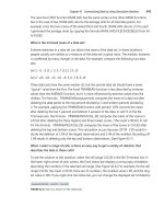
556 Microsoft Excel 2010: Data Analysis and Business Modeling
FIGURE 69-6 Using the Series dialog box to ll in the trial numbers 1 through 1,000.
Next I enter the possible production quantities (10,000, 20,000, 40,000, 69,000) in cells
B15:E15. I want to calculate prot for each trial number (1 through 1,000) and each
production quantity. I refer to the formula for prot (calculated in cell C11) in the upper-left
cell of the data table (A15) by entering =C11.
You can now trick Excel into simulating one thousand iterations of demand for each
production quantity. Select the table range (A15:E1014), and then in the Data Tools group
on the Data tab, click What If Analysis, and then select Data Table. To set up a two-way data
table, choose the production quantity (cell C1) as the row input cell and select any blank cell
(I chose cell I14) as the column input cell. After you click OK, Excel simulates one thousand
demand values for each order quantity.
To understand why this works, consider the values placed by the data table in the cell range
C16:C1015. For each of these cells, Excel uses a value of 20,000 in cell C1. In C16, the column
input cell value of 1 is placed in a blank cell, and the random number in cell C2 recalculates.
The corresponding prot is then recorded in cell C16. Then the column input cell value of 2
is placed in a blank cell, and the random number in C2 again recalculates. The corresponding
prot is entered in cell C17.
By copying from cell B13 to C13:E13 the formula AVERAGE(B16:B1015), you can compute
average simulated prot for each production quantity. By copying from cell B14 to C14:E14
the formula STDEV(B16:B1015), you can compute the standard deviation of the simulated
prots for each order quantity. Each time you press F9, one thousand iterations of demand
are simulated for each order quantity. Producing 40,000 cards always yields the largest
expected prot, so producing 40,000 cards appears to be the proper decision.
Chapter 69 Introduction to Monte Carlo Simulation 557
The Impact of Risk on Our Decision
If you produce 20,000 instead of 40,000 cards, the expected prot drops approximately 22
percent, but risk (as measured by the standard deviation of prot) drops almost 73 percent.
Therefore, if you are extremely averse to risk, producing 20,000 cards might be the right
decision. Incidentally, producing 10,000 cards always has a standard deviation of 0 cards
because if you produce 10,000 cards, you will always sell all of them without any leftovers.

Note In this workbook I set the Calculation option to Automatic Except For Tables. (Use the
Calculation command in the Calculation group on the Formulas tab.) This setting ensures that the
data table does not recalculate unless you press F9, which is a good idea because a large data
table will slow down your work if it recalculates every time you type something in your work-
sheet. Note that in this example, whenever you press F9, the mean prot changes. This happens
because each time you press F9, a different sequence of one thousand random numbers is used
to generate demands for each order quantity.
Condence Interval for Mean Prot
A natural question to ask in this situation is, Into what interval will I be 95 percent sure
that the true mean prot will fall? This interval is called the 95 percent condence interval
for mean prot. A 95 percent condence interval for the mean of any simulation output is
c omputed by the following formula:
Mean Profit
+
_
1.96 * profitst.dev.
number iterations
In cell J11, I computed the lower limit for the 95 percent condence interval on mean prot
when 40,000 calendars are produced with the formula D13–1.96*D14/SQRT(1000). In cell
J12, I computed the upper limit for the 95 percent condence interval with the formula
D13+1.96*D14/SQRT(1000). These calculations are shown in Figure 69-7.
FIGURE 69-7 Ninety-ve percent condence interval for mean prot when 40,000 calendars are ordered.
You can be 95 percent sure that your mean prot when 40,000 calendars are ordered is
between $55,076 and $61,008.
558 Microsoft Excel 2010: Data Analysis and Business Modeling
Problems
1. An auto dealer believes that demand for 2015 model cars will be normally distributed
with a mean of 200 and a standard deviation of 30. His cost of receiving an Envoy is
$25,000, and he sells an Envoy for $40,000. Half of all the Envoys not sold at full price
can be sold for $30,000. He is considering ordering 200, 220, 240, 269, 280, or 300

Envoys. How many should he order?
2. A small supermarket is trying to determine how many copies of People magazine it
should order each week. The owner believes the demand for People is governed by the
following discrete random variable:
Demand Probability
15 0.10
20 0.20
25 0.30
30 0.25
35 0.15
The supermarket pays $1.00 for each copy of People and sells it for $1.95. Each unsold
copy can be returned for $0.50. How many copies of People should the store order?
559
Chapter 70
Calculating an Optimal Bid
Questions answered in this chapter:
■
How do I simulate a binomial random variable?
■
How can I determine whether a continuous random variable should be modeled as a
normal random variable?
■
How can I use simulation to determine the optimal bid for a construction project?
When bidding against competitors on a project, the two major sources of uncertainty are
the number of competitors and the bids submitted by each competitor. If your bids are high,
you’ll make a lot of money on each project, but you’ll get very few projects. If your bids are
low, you’ll work on lots of projects but make very little money on each one. The optimal
bid is somewhere in the middle. Monte Carlo simulation is a useful tool for determining
the bid that maximizes expected prot.
Answers to This Chapter’s Questions

How do I simulate a binomial random variable?
The formula BINOM.INV(n,p,rand()) simulates the number of successes in n independent
trials, each of which has a probability of success equal to p. As explained in Chapter 69,
“Introduction to Monte Carlo Simulation,” the RAND function generates a number equally
likely to assume any value between 0 and 1. As shown in the le Binomialsim.xlsx (see
Figure 70-1), when you press F9, the formula BINOM.INV(100,0.9,D3) entered in cell C3
simulates the number of free throws that Steve Nash (a 90-percent foul shooter in the NBA)
makes in 100 attempts. The formula BINOM.INV(100,0.5,D4) in cell C4 simulates the num-
ber of heads tossed in 100 tosses of a fair coin. In cell C5, the formula BINOM.INV(3,0.4,D5)
simulates the number of competitors entering the market during a year in which there are
three possible entrants and each competitor is assumed to have a 40 percent chance of
entering the market. Of course, in D3:D5, I entered the formula RAND().
560 Microsoft Excel 2010: Data Analysis and Business Modeling
FIGURE 70-1 Simulating a binomial random variable.
How can I determine whether a continuous random variable should be modeled as a
normal random variable?
Let’s suppose that you think the most likely bid by a competitor is $50,000. Recall that the
normal probability density function (pdf) is symmetric about its mean. Therefore, to deter-
mine whether a normal random variable can be used to model a competitor’s bid, you need
to test for symmetry about the bid’s mean. If the competitor’s bid exhibits symmetry about
the mean of $50,000, bids of $40,000 and $60,000, $45,000 and $55,000, and so on should
be approximately equally likely. If the symmetry assumption seems reasonable, you can then
model each competitor’s bid as a normal random variable with a mean of $50,000.
How can you estimate the standard deviation of each competitor’s bid? Recall from the
rule of thumb discussed in Chapter 42, “Summarizing Data by Using Descriptive Statistics,”
that data sets with symmetric histograms have roughly 95 percent of their data within two
standard deviations of the mean. Similarly, a normal random variable has a 95 percent
probability of being within two standard deviations of its mean. Suppose that you are 95
percent sure that a competitor’s bid will be between $30,000 and $70,000. This implies that
2*(standard deviation of competitor’s bid) equals $20,000, or the standard deviation of a

competitor’s bid equals $10,000.
If the symmetry assumption is reasonable, you can now simulate a competitor’s bid with the
formula NORM.INV(rand(),50000,10000). (See Chapter 69 for details about how to model
normal random variables using the NORM.INV function.)
How can I use simulation to determine the optimal bid for a construction project?
Let’s assume that you’re bidding on a construction project that will cost you $25,000 to
complete. It costs $1,000 to prepare your bid. You have six potential competitors, and you
estimate that there is a 50-percent chance that each competitor will bid on the project. If a
competitor places a bid, its bid is assumed to follow a normal random variable with a mean
equal to $50,000 and a standard deviation equal to $10,000. Also suppose you are only
preparing bids that are exact multiples of $5,000. What should you bid to maximize expected
Chapter 70 Calculating an Optimal Bid 561
prot? Remember, the low bid wins! You’ll nd the work for this question in the le
Bidsim.xlsx, shown in Figures 70-2 and 70-3.
FIGURE 70-2 Bidding simulation model.
FIGURE 70-3 Bidding simulation data table.
Your strategy should be as follows:
■
Generate the number of bidders.
■
For each potential bidder who actually bids, use the normal random variable to
model the bid. If a potential bidder does not bid, you assign a large bid (for example,
$100,000) to ensure that they do not win the bidding.
■
Determine whether you are the low bidder.
562 Microsoft Excel 2010: Data Analysis and Business Modeling
■
If you are the low bidder, you earn a prot equal to your bid, less project cost, less
$1,000 (the cost of making the bid). If you are not the low bidder, you lose the $1,000
cost of the bid.

■
Use a two-way data table to simulate each possible bid (for example, $30,000,
$35,000, … $60,000) one thousand times, and then choose the bid with the largest
expected prot.
To begin, I assigned the names in the cell range D1:D4 to the range E1:E4. I determine in cell
E3 the number of bidders with the formula BINOM.INV(6,0.5,F3). Cell F3 contains the RAND()
formula. Next I determine which of the potential bidders actually bid by copying from E9 to
E10:E14 the formula IF(D9<=Number_bidders,”yes”,”no”).
I then generate a bid for each bidder (nonbidders are assigned a bid of $100,000) by copying
from cell F9 to F10:F14 the formula IF(E9=”yes”,NORM.INV(G9,50000,10000),100000).
Each cell in the cell range G9:G14 contains the RAND function. In cell D17, I determine
whether I am the low bidder and win the project with the formula
IF(mybid<=MIN(F9:F14),”yes”,”no”). In cell D19, I compute prot with the formula
IF(D17=”yes”,mybid–costproject–cost_ bid,–cost_bid), recognizing that I receive only the
amount of the bid and pay project costs if I win the bid.
Now I can use a two-way data table (shown in Figure 70-3) to simulate one thousand bids
between $30,000 and $60,000. I copy the prot to cell D22 by entering the formula =D19.
Then I select the table range D22:K1022. On the Data tab, in the Data Tools group, I click
What-If Analysis and then click Data Table to specify the input values for the data table. The
column input cell is any blank cell in the worksheet, and the row input cell is E4 (the location
of the bid). Clicking OK in the Data Table dialog box simulates the prot from each bid one
thousand times.
Copying from E21 to F21:K21 the formula AVERAGE(E23:E1022) calculates the mean prot for
each bid. Each time I press F9, I see that the mean prot for one thousand trials is maximized
by bidding $40,000.
Problems
1. How would the optimal bid change if you had 12 competitors?
2. Suppose you are bidding for an oil well that you believe will yield $40 million ( including
the cost of developing and mining the oil) in prots. Three competitors are bidding
against you, and each competitor’s bid is assumed to follow a normal random variable

with a mean of $30 million and a standard deviation of $4 million. What should you bid
(within $1 million)?
Chapter 70 Calculating an Optimal Bid 563
3. A commonly used continuous random variable is the uniform random variable. A
uniform random variable—written as U(a,b)—is equally likely to assume any value be-
tween two given numbers a and b. Explain why the formula a+(b–a)*RAND() can be
used to simulate U(a,b).
4. Investor Peter Fischer is bidding to take over a biotech company. The company is
equally likely to be worth any amount between $0 and $200 per share. Only the
company itself knows its true value. Peter is such a good investor that the market will
immediately estimate the rm’s value at 50 percent more than its true value. What
should Peter bid per share for this company?
5. Seattle Mariner baseball player Ichiro Suzuki is asking for salary arbitration on his
contract. Salary arbitration in Major League Baseball works as follows: The player
submits a salary that he thinks he should be paid, as does the team. The arbitrator
(without seeing the salaries submitted by the player or the team) estimates a fair salary.
The player is then paid the submitted salary that is closer to the arbitrator’s estimate.
For example, suppose Ichiro submits a $12 million offer, and the Seattle Mariners sub-
mit a $7 million offer. If the arbitrator says a fair salary is $10 million, Ichiro will be paid
$12 million, whereas if the arbitrator says a fair salary is $9 million, Ichiro will be paid
$7 million. Assume that the arbitrator’s estimate is equally likely to be anywhere
between $8 and $11 million, and the team’s offer is equally likely to be anywhere be-
tween $6 million and $9 million. Within $1 million, what salary should Ichiro submit?
565
Chapter 71
Simulating Stock Prices and Asset
Allocation Modeling
Questions answered in this chapter:
■
I recently bought 100 shares of GE stock. What is the probability that during the next

year this investment will return more than 10 percent?
■
I’m trying to determine how to allocate my investment portfolio between stocks,
T-Bills, and bonds. What asset allocation over a ve-year planning horizon will yield an
expected return of at least 10 percent and minimize risk?
The last few years have shown that future returns on investments are highly uncertain. In
Chapter 68, I showed how to use the lognormal random variable to model stock prices.
Many nancial experts have been critical of using the lognormal random variable to model
stock prices because the lognormal underestimates the probability of extreme events (often
called “black swans”). In this chapter, I’ll explain a relatively simple approach to assessing
uncertainty in future investment returns. This approach is based on the idea of bootstrapping.
Essentially, bootstrapping simulates future investment returns by assuming that the future
will be similar to the past. For example, if you want to simulate the stock price of GE in one
year, you can assume that each month’s percentage change in price is equally likely to be
one of, for example, the percentage changes for the previous 60 months. This method allows
you to easily generate thousands of scenarios for the future value of your investments. In
addition to scenarios that assume that future variability and average returns will be similar to
the recent past, you can easily adjust bootstrapping to reect a view that future returns on
investments will be less or more favorable than in the recent past.
After you’ve generated future scenarios for investment returns, it’s a simple matter to use
the Microsoft Excel Solver to work out the asset allocation problem—that is, how should you
allocate your investments to attain the level of expected return you want but with minimum
risk?
The following two examples demonstrate the simplicity and power of the bootstrapping
approach.
566 Microsoft Excel 2010: Data Analysis and Business Modeling
Answers to This Chapter’s Questions
I recently bought 100 shares of GE stock What is the probability that during the next
year this investment will return more than 10 percent?
Let’s suppose that GE stock is currently selling for $28.50 per share. Data for the monthly

returns on GE (as well as for Microsoft and Intel) for the months between August 1997 and
July 2002 is included in the le Gesim.xlsx, shown in Figure 71-1. For example, in the month
ending on August 2, 2002 (basically, this is July 2002), GE lost 12.1 percent. These returns
include dividends (if any) paid by each company.
FIGURE 71-1 GE, Microsoft, and Intel stock data.
The price of GE stock in one year is uncertain, so how can you get an idea about the range
of variation in the price of GE stock one year from now? The bootstrapping approach sim-
ply estimates a return on GE during each of the next 12 months by assuming that the re-
turn during each month is equally likely to be any of the returns for the 60 months listed.
In other words, the return on GE next month is equally likely to be any of the numbers in
the cell range F5:F64. To implement this idea, you use the formula RANDBETWEEN(1,60) to
choose a “scenario” for each of the next 12 months. For example, if this function returns 7
for next month, you use the return for GE in cell F11 (4.1 percent), which is the seventh cell in
the range, as next month’s return. The results are shown in Figure 71-2. (You’ll see different
values because the RANDBETWEEN function automatically recalculates random values when
you open the worksheet.)
Chapter 71 Simulating Stock Prices and Asset Allocation Modeling 567
To begin, you enter GE’s current price per share ($28.50) in cell J6. Then you generate
a scenario for each of the next 12 months by copying from K6 to K7:K17 the formula
RANDBETWEEN(1,60). Next you use a lookup table to obtain the GE return based on your
scenario. To do this, you simply copy from L6 to L7:L17 the formula VLOOKUP(K6,lookup,5).
As the formula indicates, the range B5:F64 is named Lookup, with the returns for GE in
the fth column of the lookup range. In the scenarios shown in Figure 71-2, you can see,
for example, that the return for GE twelve months into the future is equal to the 7/1/2001
data point, that is, a -10.9 percent return. (Compare cell L17 in Figure 71-2 with cell F18 in
Figure 71-1.)
FIGURE 71-2 Simulating GE stock price in one year.
Copying from M6 to M7:M17 the formula (1+L6)*J6 determines each month’s ending GE
price. The formula takes the form (1+ month’s return)*(GE’s beginning price). Finally, copying
from J7 to J8:J17 the formula =M6 computes the beginning price for each month as equal to

the previous month’s ending price.
You can now use a data table to generate one thousand scenarios for GE’s price in one
year and the one-year percentage return on your investment. The data table is shown in
Figure 71-3. In cell J19, you copy the ending price with the formula =M17. In cell K19, you
enter the formula (M17–$J$6)/$J$6 to compute the one-year return as (Ending GE price–
Beginning GE price)/Beginning GE price.
568 Microsoft Excel 2010: Data Analysis and Business Modeling
FIGURE 71-3 Data table for GE simulation.
Next, select the table range (J19:K1019), click What-If Analysis in the Data Tools group on the
Data tab, and then select Data Table. You set up a one-way data table by selecting a blank
cell as the column input cell. After you click OK in the Data Table dialog box, Excel generates
one thousand scenarios for GE’s stock price in one year. (The calculation option for this work-
book has been set to Automatic Except For Tables on the Formulas tab in the Excel Options
dialog box. You need to press F9 if you want to see the simulated prices change.)
In cells M20:M24, I used the COUNTIF function (see Chapter 20, “The COUNTIF, COUNTIFS,
COUNT, COUNTA, and COUNTBLANK Functions”) to summarize the range of returns that can
occur in one year. For example, in cell M20, I computed the probability of losing money in
one year with the formula COUNTIF(returns,”<0”)/1000. (I named the range containing the
one thousand simulated returns as Returns.) The simulation indicates that, based on the data
for 1997–2002, there is roughly a 40-percent chance that our GE investment will lose money
during the next year. You can also see the following results:
■
There is a 45-percent probability that returns will be more than 10 percent.
■
There is a 15-percent probability that returns will be between 0 and 10 percent.
■
There is a 12-percent chance that the investment will lose between 0 and 10 percent.
■
There is a 28-percent chance that the investment will lose more than 10 percent.
■

The average return for the next year will be approximately 10.7 percent.
Many pundits believe that future stock returns will not be as good as in the recent past.
Suppose you feel that in the next year, GE will perform on average 5 percent worse per year
than it performed during the 1997–2002 period for which you have data. You can easily in-
corporate this assumption into a simulation by changing the nal price formula for GE in cell
M17 to (1+L17)*J17–0.05*J6. This simply reduces the ending GE price by 5 percent of its initial
price, which reduces your returns for the next year by 5 percent. You can see these results in
the le Gesimless5.xlsx, shown in Figure 71-4.
Chapter 71 Simulating Stock Prices and Asset Allocation Modeling 569
FIGURE 71-4 Pessimistic view of the future.
Note that the estimate is now a 50-percent chance that the price of GE stock will decrease
during the next year. The average is not exactly 5 percent lower than the previous simulation
because each time you run one thousand iterations, the simulated values change.
I’m trying to determine how to allocate my investment portfolio between stocks, T-Bills,
and bonds What asset allocation over a ve-year planning horizon will yield an annual
expected return of at least 8 percent and minimize risk?
A key decision made by individuals, mutual fund managers, and other investors is how to
allocate assets between different asset classes given the future uncertainty about returns
for these asset classes. A reasonable approach to asset allocation is to use bootstrapping
to generate one thousand simulated values for the future values of each asset class, and
then use the Excel Solver to determine an asset allocation that yields an expected return yet
minimizes risk. As an example, suppose you are given annual returns on stocks, T-Bills, and
bonds during the period 1973–2009. You are investing for a ve-year planning horizon, and
based on the historical data, you want to know which asset allocation yields a minimum risk
(as measured by standard deviation) of annual returns and yields an annual expected return
of at least 10 percent. You can see this data in the le Assetallsim.xlsx, shown in Figure 71-5.
(Not all the data is shown.)
FIGURE 71-5 Historical returns on stocks, T-Bills, and bonds.
570 Microsoft Excel 2010: Data Analysis and Business Modeling
To begin, you use bootstrapping to generate one thousand simulated values for stocks,

T-Bills, and bonds in ve years. Assume that each asset class has a current price of $1.
(See Figure 71-6.)
For each asset class, you enter an initial unit price of $1 in the cell range H10:J10. Next, by
copying from K10 to K11:K14 the formula RANDBETWEEN(1973,2009), you generate a
scenario for each of the next ve years. For example, for the data shown, next year will be
similar to 1985; the following year will be similar to 1986, and so on. Copying from L10 to
L10:N14 the formula H10*(1+VLOOKUP($K10,lookup,L$8)) generates each year’s ending value
for each asset class. For stocks, for example, this formula computes the following:
(Endingyeartstockvalue)=(Beginningyeartstockvalue)*(1+Yeartstockreturn)
FIGURE 71-6 Simulating ve-year returns on stocks, T-Bills, and bonds.
Copying from H11 to H11:J14 the formula =L10 computes the value for each asset class at
the beginning of each successive year.
You can now use a one-way data table to generate one thousand scenarios of the value of
stocks, T-Bills, and bonds in ve years. Begin by copying the Year 5 ending value for each as-
set class to cells I16:K16. Next select the table range (H16:K1015), click What If Analysis on the
Data tab, and then click Data Table. Use any blank cell as the column input cell to set up a
one-way data table. After clicking OK in the Data Table dialog box, you obtain one thousand
simulated values for the value of stocks, T-Bills, and bonds over ve years. It is important to
note that this approach models the fact that stocks, T-Bills, and bonds do not move indepen-
dently. In each of the ve years, the stock, T-Bill, and bond returns are always chosen from
the same row of data. This enables the bootstrapping approach to reect the interdepen-
dence of returns on these asset classes that has been exhibited during the recent past. (See
Problem 7 at the end of this chapter for concrete evidence that bootstrapping appropriately
models the interdependence between the returns on our three asset classes.)
Chapter 71 Simulating Stock Prices and Asset Allocation Modeling 571
With this setup, we’re ready to nd the optimal asset allocation, which I calculated in the le
Assetallocationopt.xlsx, shown in Figure 71-7. To start, I copy the one thousand simulated
ve-year asset values and paste them into a blank worksheet (I used the cell range C4:E1003).
In cells C2:E2, I enter trial fractions of our assets allocated to stocks, T-Bills, and bonds,
respectively. In cell F2, I add these asset allocation fractions with the formula SUM(C2:E2).

Later, I’ll add the constraint F2=1 to the Solver model, which ensures that I invest 100 percent
of our money in one of the three asset classes.
FIGURE 71-7 Optimal asset allocation model.
Next I want to determine the nal portfolio value for each scenario. To make this calculation,
I can use a formula such as (Final portfolio value)=(Final value of stocks)+
(Final value of T-bills)+(Final value of bonds). Copying from cell F4 to F5:F1003 the formula
SUMPRODUCT(C4:E4,$C$2:$E$2) determines the nal asset position for each scenario.
The next step is to determine the annual return over the ve-year simulated period for each
scenario that Excel generated. Note that (1+ Annual return)
5
equals (Final portfolio value)/
(Initial portfolio value). Because the initial portfolio value is just $1, this tells you that
Annual return equals (Final portfolio value)
1/5
–1.
By copying from cell G4 to G5:G1003 the formula (F4/1)^(1/5)–1, I compute the annual
return for each scenario during the ve-year simulated period. After naming the range
G4:G1003 (which contains the simulated annual returns) as Returns, I compute the average
annual return in cell I3 with the formula AVERAGE(returns) and the standard deviation of the
annual returns in cell I4 with the formula STDEV.S(returns).
Now I’m ready to use Solver to determine the set of allocation weights that yields an
expected annual return of at least 8 percent yet minimizes the standard deviation of the
annual returns. The Solver Parameters dialog box set up to perform this calculation is shown
in Figure 71-8.
572 Microsoft Excel 2010: Data Analysis and Business Modeling
FIGURE 71-8 Solver Parameters dialog box set up for our asset allocation model.
■
I try to minimize the standard deviation of the annual portfolio return (cell I4).
■
The changing cells are the asset allocation weights (cells C2:E2).

■
I must allocate 100 percent of the money I have to the three asset classes (F2=1).
■
The expected annual return must be at least 8 percent (I3>=0.08).
■
I assume that no short sales are allowed, which is modeled by forcing the fraction of
the money in each asset class to be nonnegative. To implement this, I selected the
Make Unconstrained Variables Non-Negative check box.
■
The minimum risk asset allocation is 24.3 percent stocks, 75.7 percent T-Bills, and no
bonds. This portfolio yields an expected annual return of 8 percent and an annual
standard deviation of 2.3 percent.
Suppose you believe that the next 5 years will, on average, produce returns for stocks that
are 5 percent worse than they’ve been for the last 30 years. It is easy to incorporate these
expectations into the simulation. (See Problem 4 at the end of the chapter.)
Chapter 71 Simulating Stock Prices and Asset Allocation Modeling 573
Problems
Problems 1-3 utilize data in the le Gesim.xlsx.
1. Assume that the current price of Microsoft stock is $28 per share. What is the
probability that in two years the price of Microsoft stock will be at least $35?
2. Solve Problem 1 again, but this time with the assumption that during the next two
years, Microsoft will on average perform 6 percent better per year than it performed
during the 1997–2002 period for which you have data.
3. Assume that the current price of Intel is $20 per share. What is the probability that
during the next three years, you will earn at least a 30-percent return (for the three-
year period) on a purchase of Intel stock?
Problems 4 through 7 utilize data in the le Assetallsim.xlsx.
4. Suppose you believe that over the next ve years, stocks will produce returns that are
5 percent worse per year, on average, than the 1973–2009 data. Find an asset alloca-
tion between stocks, T-Bills, and bonds that yields an expected annual return of at least

6 percent yet minimizes risk.
5. Suppose you believe that it is two times more likely that investment returns for each of
the next ve years will be more like the period 1992–2001 than the period 1972–1991.
For example, the chance that next year will be like 1993 has twice the probability
that next year will be like 1980. This belief causes your bootstrapping analysis to give
more weight to the recent past. How would you factor this belief into your portfolio
optimization model?
6. Many mutual funds and investors hedge the risk that stocks will go down by purchasing
put options. (See Chapter 74, “Pricing Stock Options,” for more discussion of put
options.) How could an asset allocation model be used to determine an optimal
hedging strategy that uses puts?
7. Determine the correlations (based on the 1973–2009 data) between annual returns on
stocks, T-Bills, and bonds. Then determine the correlation (based on the one thousand
scenarios created by bootstrapping) between the nal values for stocks, T-Bills, and
assets. Does it appear that the bootstrapping approach picks up the interdependence
between the returns on stocks, T-Bills, and bonds?
575
Chapter 72
Fun and Games: Simulating
Gambling and Sporting Event
Probabilities
Questions answered in this chapter:
■
What is the probability of winning at craps?
■
In ve-card draw poker, what is the probability of getting three of a kind?
■
Going into the NCAA basketball Final Four, what is the probability of each team
winning the tournament?
Gambling and following sporting events are popular pastimes. I think gambling and sports

are exciting because you never know what’s going to happen. Monte Carlo simulation is a
powerful tool that you can use to approximate gambling and sporting event probabilities.
Essentially, you estimate probability by playing out a gambling or sporting event situation
multiple times. If, for example, you have Microsoft Excel play out the game of craps 10,000
times and you win 4,900 times, you would estimate the probability of winning at craps to
equal 4900/10,000, or 49 percent. If you play out the 2003 NCAA men’s Final Four 1,000
times and Syracuse wins 300 of the iterations, you would estimate Syracuse’s probability of
winning the championship as 300/1,000, or 30 percent.
Answers to This Chapter’s Questions
What is the probability of winning at craps?
In the game of craps, a player rolls two dice. If the combination is 2, 3, or 12, the player loses.
If the combination is 7 or 11, the player wins. If the combination is a different number, the
player continues rolling the dice until he or she either matches the number thrown on the
rst roll (called the point) or rolls 7. If the player rolls the point before rolling 7, the player
wins. If the player rolls 7 before rolling the point, the player loses. By complex calcula-
tions, you can show that the probability of a player winning at craps is 0.493. You can use
Excel to simulate the game of craps many times (I chose two thousand) to approximate this
probability.
In this example, it is crucial to keep in mind that you don’t know how many rolls the game
will take. I will show that the chance of a game requiring more than 50 rolls of the dice is
576 Microsoft Excel 2010: Data Analysis and Business Modeling
highly unlikely, so we’ll play out 50 rolls of the dice. After each roll, the game status is tracked
as follows:
■
0 equals the game is lost.
■
1 equals the game is won.
■
2 equals the game continues.
The output cell keeps track of the status of the game after the ftieth roll by recording 1 to

indicate a win and 0 to indicate a loss. You can review the work I did in the le Craps.xlsx,
shown in Figure 72-1.
FIGURE 72-1 Simulating a game of craps.
In cell B2, I used the RANDBETWEEN function to generate the number on the rst die on the
rst roll by using the formula RANDBETWEEN(1,6). The RANDBETWEEN function ensures
that each of its arguments is equally likely, so each die has an equal (1/6) chance of yielding
1, 2, 3, 4, 5, or 6. Copying this formula to the range B2:AY3 generates 50 rolls of the dice. (In
Figure 72-1, I hid rolls 8 through 48.)
In the cell range B4:AY4, I compute the total dice combination for each of the 50 rolls by
copying from B4 to C4:AY4 the formula SUM(B2:B3). In cell B5, I determine the
game status
after the rst roll with the formula IF(OR(B4=2,B4=3,B4=12),0,IF(OR(B4=7,B4=11),1,2)).
Remember that a roll of 2, 3, or 12 results in a loss (entering 0 in the cell); a roll of 7 or 11
results in a win (1); and any other roll results in the game continuing (2).
Chapter 72 Fun and Games: Simulating Gambling and Sporting Event Probabilities 577
In cell C5, I compute the status of the game after the second roll with the formula
IF(OR(B5=0,B5=1),B5,IF(C4=$B4,1,IF(C4=7,0,2))). If the game ends on the rst roll, I maintain
the status of the game. If a roll makes our point, I record a win with 1. If a roll is a 7, I record
a loss. Otherwise, the game continues. I added a dollar sign in the reference to column B
($B4) in this formula to ensure that each roll tries to match the point thrown on the rst roll.
Copying this formula from C5 to D5:AY5 records the game status after rolls 2 through 50.
The game result is in cell AY5, which is copied to C6 so that you can easily see it. I then use
a one-way data table to play out the game of craps two thousand times. In cell E9 I enter
the formula =C6, which tracks the nal outcome of the game (0 if a loss or 1 if a win). Next, I
select the table range (D9:E2009), click What-If Analysis in the Data Tools group on the Data
tab, and then click Data Table. I choose a one-way table with any blank cell as the column
input cell. After I press F9, Excel simulates the game of craps two thousand times.
In cell E8, I can compute the fraction of the simulations that result in wins with the formula
AVERAGE(E10:E2009). For the two thousand iterations, I won 49.25 percent of the time. If
I had run more trials (for example, 10,000 iterations), I would have come closer to the true

probability of winning at craps (49.3%). For information about using a one-way data table,
see Chapter 17, “Sensitivity Analysis with Data Tables.”
In ve-card draw poker, what is the probability of getting three of a kind?
An ordinary deck of cards contains four cards of each type—four aces, four deuces, and
so on, up to four kings. To estimate the probability of getting a particular poker hand, you
can assign the value 1 to an ace, 2 to a deuce, and on up through the deck so that a jack is
assigned the value 11, a queen is assigned 12, and a king is assigned 13.
In ve-card draw poker, you are dealt ve cards. Many probabilities are of interest, but let’s
use simulation to estimate the probability of getting three of a kind, which requires that you
have three of one type of card and no pairs. (If you have a pair and three of a kind, the hand
is a full house.) To simulate the ve cards drawn, you proceed as follows. (See the le
Poker.xlsx, shown in Figure 72-2.)
■
Associate a random number with each card in the deck.
■
The ve cards chosen will be the ve cards associated with the ve smallest random
numbers, which gives each card an equal chance of being chosen.
■
Count how many of each card (ace through king) are drawn.
578 Microsoft Excel 2010: Data Analysis and Business Modeling
FIGURE 72-2 Estimating the probability that you’ll draw three of a kind in a poker game.
To begin, I list in cells D3:D54 all the cards in the deck: four 1s, four 2s, and so on up to
four 13s. Then I copy from cell E3 to E4:E54 the RAND function to associate a random
number with each card in the deck. Copying from C3 to C4:C54 the formula
RANK.EQ(E3,$E$3:$E$54,1) gives the rank (ordered from smallest to largest) of each
random number. For example, in Figure 72-2, you can see that the rst 3 in the deck (row 11)
is associated with the fourteenth smallest random number. (You will see different results in
the worksheet because the random numbers are automatically recalculated when you open
the worksheet.)
The syntax of the RANK.EQ function is RANK.EQ(number,array,1 or 0). If the last argument of

the RANK.EQ function is 1, the function returns the rank of the number in the array with the
smallest number receiving a rank of 1, the second smallest number a rank of 2, and so on. If
the last argument of the RANK.EQ function is 0, the function returns the rank of the num-
ber in the array with the largest number receiving a rank of 1, the second largest number
receiving a rank of 2, and so on.
In ranking random numbers, no ties can occur (because the random numbers would have to
match 16 digits).
Chapter 72 Fun and Games: Simulating Gambling and Sporting Event Probabilities 579
Suppose, for example, that you are ranking the numbers 1, 3, 3, and 4 and that the last
argument of the RANK.EQ function was 1. Excel would return the following ranks:
Number Rank (smallest number has rank of 1)
1 1
3 2
3 2
4 4
Because 3 is the second smallest number, 3 would be assigned a rank of 2. The other 3 would
also be assigned a rank of 2. Because 4 is the fourth smallest number, it would be assigned
a rank of 4. Understanding the treatment of ties by the RANK.EQ function will help you
complete Problem 1 at the end of the chapter.
By copying from cell B3 to B4:B7 the formula VLOOKUP(A3,lookup,2,FALSE), you can draw
ve cards from the deck. This formula draws the ve cards corresponding to the ve smallest
random numbers. (The lookup table range C3:D54 has been named Lookup.) I used FALSE in
the VLOOKUP function because the ranks need not be in ascending order.
Having assigned the range name Drawn to the drawn cards (the range B3:B7), copying from
J3 to J4:J15 the formula COUNTIF(drawn,I3) counts how many of each card are in the hand
drawn. In cell J17, I determine whether the hand includes three of a kind with the formula IF
(AND(MAX(J3:J15)=3,COUNTIF(J3:J15,2)=0),1,0). This formula returns a 1 if and only if the
hand has three of one kind and no pairs.
I now use a one-way data table to simulate four thousand poker hands. In cell J19, I recopy
the results of cell J17 with the formula

J17. Next I select the table range (I19:J4019). After
clicking What-If Analysis in the Data Tools group on the Data tab and then clicking Data
Table, I set up a one-way data table by selecting any blank cell as the column input cell. After
I click OK, Excel simulates four thousand poker hands. In cell G21, I record the estimated
probability of three of a kind with the formula AVERAGE(J20:J4019). I estimate the chance
of three of a kind at 1.9 percent. (Using basic probability theory, you can show that the true
probability of drawing three of a kind is 2.1 percent.)
Going into the 2003 NCAA men’s basketball Final Four, what was the probability of each
team winning the tournament?
You can rate college basketball teams using the methodology described in Chapter 34,
“Using Solver to Rate Sports Teams,” but it is difcult to get the scores of all past games. The
highly respected Sagarin ratings (available at www.usatoday.com/sports/sagarin.htm) always
gives up-to-date ratings for all college basketball teams. On the eve of the 2003 men’s Final
Four, the Sagarin ratings of the four teams were Syracuse (led by Carmelo Anthony), 91.03;
Kansas, 92.76; Marquette (led by Dwayne Wade), 89.01; and Texas, 90.66. Given this informa-
tion, you can play out the Final Four several thousand times to estimate the chance that each
team will win.
580 Microsoft Excel 2010: Data Analysis and Business Modeling
The mean prediction for the number of points by which the home team wins is favorite
rating–underdog rating. In the Final Four, there is no home team, but if there was one, you
would add ve points to the home team’s rating. (In professional basketball, the home edge
is four points, and in college and professional football, the home edge is three points.) Then
you can use the NORM.INV function to simulate the outcome of each game. (See Chapter 65,
“The Normal Random Variable,” for a discussion of using the NORMINV function to simulate
a normal random variable.)
I calculated the likely outcome of the 2003 Final Four in the le Final4sim.xlsx, shown in
Figure 72-3. The seminals pitted Kansas against Marquette and Syracuse against Texas.
FIGURE 72-3 Simulating the outcome of the NCAA 2003 Final Four.
To begin, I enter each team’s name and rating in the cell range C4:D5 and C8:D9. In cell F4,
I use the RAND function to enter a random number for the Marquette–Kansas game, and

in cell F8 I enter a random number for the Syracuse–Texas game. The simulated outcome is
always relative to the top team listed.
In cell E4, I determine the outcome of the Kansas–Marquette game (from the standpoint of
Kansas) with the formula NORM.INV(F4,D4–D5,10). Note that Kansas is favored by D4–D5
points. In cell E8, I determine the outcome of the Texas–Syracuse game (from the standpoint
of Syracuse) with the formula NORM.INV(F8,D8–D9,10). (The standard deviation for the
winning margin of college basketball games is 10 points.)
In cells G5 and G6, I ensure that the winner of each seminal game moves on to the nals. A
seminal outcome of greater than 0 causes the top listed team to win; otherwise, the bottom
listed team wins. Thus, in cell G5, I enter the winner of the rst game by using the formula
Chapter 72 Fun and Games: Simulating Gambling and Sporting Event Probabilities 581
IF(E4>0,”KU”, “MARQ”). In cell G6, I enter the winner of the second game by using the
formula IF(E8>0,”SYR”,”TEX”).
In cell H5, I enter a random number that is used to simulate the outcome of the
championship game. Copying from I5 to I6 the formula VLOOKUP(G5,$C$4:$D$9,2,FALSE)
obtains the rating for each team in the championship game. Next, in cell J5, I compute the
outcome of the championship game (from the reference point of the top listed team in
cell G5) with the formula NORM.INV(H5,I5–I6,10). Finally, in cell K5, I determine the actual
champion with the formula IF(J5>0,G5,G6).
Now I can use a one-way data table in the usual fashion to play out the Final Four two
thousand times. The simulated winners are in the cell range M12:M2011. Copying from K12
to K13:K15 the formula COUNTIF($M$12:$M$2011,J12)/2000 computes the predicted prob-
ability for each team winning: 38 percent for Kansas, 24 percent for Syracuse, 24 percent for
Texas, and 14 percent for Marquette. These probabilities can be translated to odds using the
following formula:

prob team wins
prob team loses
Odds against team winning =
For example, the odds against Kansas are 1.63 to 1:

(1 – 0.38)/0.38 = 1.63
This means that if you placed $1 on Kansas to win and a bookmaker paid us $1.63 for a
Kansas championship, the bet is fair. Of course, the bookie will lower these odds slightly to
ensure that he makes money. (See Problem 6 at the end of this chapter for a related exercise.)
This methodology can easily be extended to simulate the entire NCAA tournament. Just use
IF statements to ensure that each winner advances, and use VLOOKUP functions to nd each
team’s rating. See the le Ncaa2003.xlsx for a simulation of the 2003 tournament. The analy-
sis gave Syracuse (the eventual winner) a 4-percent chance to win at the start of tournament.
In this worksheet, I used comments to explain my work, which you can see in Figure 72-4.
Here is some background about using comments:
■
To insert a comment in a cell, rst select the cell. On the Review tab, in the Comments
group, click New Comment, and then type your comment text. You will see a small red
mark in the upper-right corner of any cell containing a comment.
■
To edit a comment, right-click the cell containing the comment, and click Edit
Comment.
■
To make a comment always visible, right-click the cell, and click Show/Hide Comments.
Clicking Hide Comment when the comment is displayed hides the comment unless the
pointer is in the cell containing the comment.
582 Microsoft Excel 2010: Data Analysis and Business Modeling
■
If you want to print your comments, click the Page Setup dialog box launcher (the
small arrow in the bottom-right corner of the group) on the Page Layout tab to display
the Page Setup dialog box. In the Comments box on the Sheet tab, you can indicate
whether you want comments printed as displayed on the sheet or at the end of the
sheet.
FIGURE 72-4 Comments in a worksheet.
Problems

1. Suppose 30 people are in a room. What is the probability that at least two of them
have the same birthday?
2. What is the probability of getting dealt one pair in ve-card draw poker?
3. What is the probability of getting dealt two pairs in ve-card draw poker?
4. In the game of keno, 80 balls (numbered 1 through 80) are mixed up, and then 20 balls
are randomly drawn. Before the 20 balls are drawn, a player chooses 10 different num-
bers. If at least 5 of the numbers are drawn, the player wins. What is the probability of
winning?
5. Going into the 2003 NBA nals, the rating system described in Chapter 34 rated the
San Antonio Spurs three points higher than the New Jersey Nets. Teams play until one
team wins four games. The rst two games were at San Antonio, the next three at New
Jersey, and the nal two games were scheduled for San Antonio. What is the probabil-
ity that San Antonio will win the series?
6. What odds should the bookmaker give on Kansas winning the Final Four if the book-
maker wants to earn an average of 10 cents per dollar bet?
7. What is the probability of getting dealt a ush in ve-card draw poker?
8. If you break a 1-inch stick in two places that are randomly chosen, you have three
smaller sticks. What are the chances that the three sticks form a triangle?
9. Suppose each hitter on a baseball team has a 50-percent chance of hitting a home
run and a 50-percent chance of striking out. On average, how many runs will this team
score in an inning?