Microsoft Excel 2010: Data Analysis and Business Modeling phần 10 ppsx

628 Microsoft Excel 2010: Data Analysis and Business Modeling
For prices near the current price, however, the linear demand curve is usually a good
approximation of the product’s true demand curve.
As a second example, let’s again assume that a product is currently selling for $100 and
demand equals 500 units. The product’s price elasticity for demand is 2. Now let’s t a
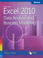
power demand curve to this information. See the le Powert.xlsx, shown in Figure 79-2.
FIGURE 79-2 Power demand curve.
In cell E3, I enter a trial value for a. Then, in cell D5, I enter the current price of $100. Because
elasticity of demand equals 2, we know that the demand curve has the form q=ap
-2
, where
a is unknown. In cell E5, I enter the demand for a price of $100, corresponding to the value
of a in cell E3, with the formula a*D5^-2. Now I can use the Goal Seek command (for details,
see Chapter 18, “The Goal Seek Command”) to determine the value of a that makes the de-
mand for price $100 equal to 500 units. I simply set cell E5 to the value 500 by changing cell
E3. I nd that a value for a of 5 million yields a demand of 500 at a price of $100. Thus, the
demand curve (graphed in Figure 79-2) is given by q=5,000,000p
-2
. For any price, the price
elasticity of demand on this demand curve equals 2.
What does a demand curve tell us about a customer’s willingness to pay for our
product?
Let’s suppose you are trying to sell a software program to a Fortune 500 company. Let q
equal the number of copies of the program the company demands, and let p equal the price
charged for the software. Suppose you have estimated that the demand curve for software
is given by q=400–p. Clearly, your customer is willing to pay less for each additional unit
of the software program. Locked inside this demand curve is information about how much
the company is willing to pay for each unit of the program. This information is crucial for
maximizing protability of sales.
Chapter 79 Estimating a Demand Curve 629
Let’s rewrite the demand curve as p=400–q. Thus, when q=1, p=$399, and so on. Now let’s

try and gure out the value the customer attaches to each of the rst two units of the pro-
gram. Assuming that the customer is rational, the customer will buy a unit if and only if the
value of the unit exceeds your price. At a price of $400, demand equals 0, so the rst unit
cannot be worth $400. At a price of $399, however, demand equals 1 unit. Therefore, the
rst unit must be worth something between $399 and $400. Similarly, at a price of $399,
the customer does not purchase the second unit. At a price of $398, however, the customer
is purchasing two units, so the customer does purchase the second unit. Therefore, the
customer values the second unit somewhere between $399 and $398.
It can be shown that the best approximation of the value of the ith unit purchased by the
customer is the price that makes demand equal to i–0.5. For example, by setting q equal to
0.5, the value of the rst unit is 400–0.5=$399.50. Similarly, by setting q=1.5, the value of the
second unit is 400–1.5=$398.50.
Problems
1. Suppose you are charging $60 for a board game you invented and have sold three
thousand copies during the last year. Elasticity for board games is known to equal 3.
Use this information to determine a linear and power demand curve.
2. For each of your answers in Problem 1, determine the value consumers place on the
two thousandth unit purchased of your game.
631
Chapter 80
Pricing Products by Using Tie-Ins
Question answered in this chapter:
■
How does the fact that customers buy razor blades as well as razors affect the
prot-maximizing price of razors?
Certain consumer product purchases frequently result in the purchase of related products,
or tie-ins. Here are some examples:
Original purchase Tie-in product
Razor Razor blades
Men’s suit Shirt and/or tie

Personal computer Software training manual
Video game console Video game
Using the techniques I described in Chapter 79, “Estimating a Demand Curve,” it’s easy to
determine a demand curve for the product that’s originally purchased. You can then use the
Microsoft Excel Solver to determine the original product price that maximizes the sum of the
prot earned from the original and the tie-in products. The following example shows how
this analysis is done.
Answer to This Chapter’s Question
How does the fact that customers buy razor blades as well as razors affect the
prot-maximizing price of razors?
Suppose that you’re currently charging $5.00 for a razor and you’re selling 6 million razors.
Assume that the variable cost of producing a razor is $2.00. Finally, suppose that the price
elasticity of demand for razors is 2. What price should you charge for razors?
Let’s assume (incorrectly) that no purchasers of razors buy blades. You determine the
demand curve (assuming a linear demand curve) as shown in Figure 80-1. (You can nd this
data and the chart on the No Blades worksheet in the le Razorsandblades.xlsx.) Two points
on the demand curve are price=$5.00, demand=6 million razors and price=$5.05 (an increase
of 1 percent), demand=5.88 million (2 percent less than 6 million). After drawing a chart and
inserting a linear trendline as shown in Chapter 79, you nd the demand curve equation is
y=18–2.4x. Because x equals price and y equals demand, you can write the demand curve for
razors as follows: demand (in millions)=18–2.4(price).
632 Microsoft Excel 2010: Data Analysis and Business Modeling
FIGURE 80-1 Determining the prot-maximizing price for razors.
I associate the names in cell C6 and the range C9:C11 with cells D6 and D9:D11. Next, I
enter a trial price in D9 and determine demand for that price in cell D10 with the formula
18-2.4*price. Then I determine in cell D11 the prot for razors by using the formula
demand*(price–unit_cost).
Next, I use Solver to determine the prot-maximizing price. The Solver Parameters dialog box
is shown in Figure 80-2.
FIGURE 80-2 Solver Parameters dialog box set up for maximizing razor prot.

I maximize the prot cell (cell D11) by changing the price (cell D9). The model is not linear
because the target cell multiplies together two quantities—demand and (price–cost)—each
Chapter 80 Pricing Products by Using Tie-Ins 633
depending on the changing cell. Solver nds that charging $4.75 for a razor maximizes prot.
(Maximum prot is $18.15 million.)
Now let’s suppose that the average purchaser of a razor buys 50 blades and that you earn
$0.15 of prot per blade purchased. How does this change the price you should charge for a
razor? Assume that the price of a blade is xed. (In Problem 3 at the end of the chapter, the
blade price changes.) The analysis is in the Blades worksheet, which is shown in Figure 80-3.
FIGURE 80-3 Price for razors with blade prot included.
I used the Create From Selection command in the Dened Names group on the Formulas
tab to associate the names in cells C6:C11 with cells D6:D11. (For example, cell D10 is named
Demand.)
Note Astute readers will recall that I also named cell D10 of the No Blades worksheet Demand.
What does Excel do when you use the range name Demand in a formula? Excel simply refers to
the cell named Demand in the current worksheet. In other words, when you use the range name
Demand in the Blades worksheet, Excel refers to cell D10 of that worksheet and not to cell D10 in
the No Blades worksheet.
In cells D7 and D8, I entered the relevant information about blades. In D9, I entered a
trial price for razors, and in D10 I computed demand with the formula 18-2.4*price. Next,
in cell D11, I computed total prot from razors and blades with the formula
demand*(price–unit_cost)+demand*blades_per_razor*prot_per_blade. Notice that
demand*blades_per_razor*prot_per_blade is the prot from blades.
The Solver setup is exactly as was shown earlier in Figure 80-2: change the price to maximize
the prot. Of course, now the prot formula includes the prot earned from blades. Excel
shows that prot is maximized by charging only $1.00 (half the variable cost!) for a razor.
This price results from making so much money from blades. You are much better off
634 Microsoft Excel 2010: Data Analysis and Business Modeling
ensuring that many people have razors even though you lose $1.00 on each razor sold. Many
companies do not understand the importance of the prot from tie-in products. This leads

them to overprice their primary product and not maximize their total prot.
Problems
Note In all of the following problems, assume a linear demand curve.
1. You are trying to determine the prot-maximizing price for a video game console.
Currently, you are charging $180 and selling 2 million consoles per year. It costs $150 to
produce a console, and price elasticity of demand for consoles is 3. What price should
you charge for a console?
2. Now assume that, on average, a purchaser of your video game console buys 10 video
games and you earn $10 prot on each video game. What is the correct price for
consoles?
3. In the razor and blade example, suppose the cost to produce a blade is $0.20. If you
charge $0.35 for a blade, a customer buys an average of 50 blades. Assume the price
elasticity of demand for blades is 3. What price should you charge for a razor and for a
blade?
4. You are managing a movie theater that can handle up to eight thousand patrons per
week. The current demand, price, and elasticity for ticket sales, popcorn, soda, and
candy are given in Figure 80-4. The theater keeps 45 percent of ticket revenues. Unit
cost per ticket, popcorn sales, candy sales, and soda sales are also given. Assuming
linear demand curves, how can the theater maximize prots? Demand for foods is the
fraction of patrons who purchase the given food.
FIGURE 80-4 Movie problem data.
5. A prescription drug is produced in the United States and sold internationally. Each unit
of the drug costs $60 to produce. In the German market, you are selling the drug for
150 euros per unit. The current exchange rate is 0.667 U.S. dollars per euro. Current
demand for the drug is 100 units, and the estimated elasticity is 2.5. Assuming a linear
demand curve, determine the appropriate sales price (in euros) for the drug.
635
Chapter 81
Pricing Products by Using
Subjectively Determined Demand

Questions answered in this chapter:
■
Sometimes I don’t know the price elasticity for a product. In other situations, I don’t
believe a linear or power demand curve is relevant. Can I still estimate a demand curve
and use Solver to determine a prot-maximizing price?
■
How can a small drugstore determine the prot-maximizing price for lipstick?
Answer to This Chapter’s Questions
Sometimes I don’t know the price elasticity for a product. In other situations, I don’t
believe a linear or power demand curve is relevant. Can I still estimate a demand
curve and use Solver to determine a prot-maximizing price?
In situations when you don’t know the price elasticity for a product or don’t think you can
rely on a linear or power demand curve, a good way to determine a product’s demand curve
is to identify the lowest price and highest price that seem reasonable. You can then try to es-
timate the product’s demand with the high price, the low price, and a price midway between
the high and low prices. Given these three points on the product’s demand curve, you can
use the Microsoft Excel trendline feature to t a quadratic demand curve with the following
formula (which I’ll call Equation 1):
Demand=a(price)
2
+b(price)+c
For any three specied points on the demand curve, values of a, b, and c exist that will make
Equation 1 exactly t the three specied points. Because Equation 1 ts three points on the
demand curve, it seems reasonable to believe that the equation will give an accurate repre-
sentation of demand for other prices. You can then use Equation 1 and Solver to determine
maximum prot, which is given by the formula (price–unit cost)*demand. The following
example shows how this process works.
How can a small drugstore determine the prot-maximizing price for lipstick?
Let’s suppose that a drugstore pays $0.90 for each unit of lipstick it orders. The store is
considering charging from $1.50 through $2.50 for a unit of lipstick. The store thinks that at a

price of $1.50, it will sell 60 units per week. (See Figure 81-1 and the le Lipstickprice.xlsx.) At
a price of $2.00, the store thinks it will sell 51 units per week, and at a price of $2.50, 20 units
per week. What price should the store charge for lipstick?
636 Microsoft Excel 2010: Data Analysis and Business Modeling
FIGURE 81-1 Lipstick pricing model.
You begin by entering the three points with which you’ll chart the demand curve in the cell
range E3:F6. After selecting E3:F6, click the Charts group on the ribbon’s Insert tab, and then
select the rst option for a Scatter chart. You can then right-click a data point and select Add
Trendline. In the Format Trendline dialog box (see Figure 81-2), choose Polynomial and select
2 in the Order box (to obtain a quadratic curve of the form of Equation 1). Then select the
option Display Equation On Chart.
FIGURE 81-2 Conguring the Format Trendline dialog box for selecting polynomial demand curve.
Chapter 81 Pricing Products by Using Subjectively Determined Demand 637
Excel creates the chart shown in Figure 81-1. The estimated demand curve (Equation 2) is
Demand=–44*Price
2
+136*Price–45.
Next, you insert a trial price in cell I2. You compute product demand by using Equation 2 in
cell I3 with the formula –44*price^2+136*price–45. (I named cell I2 Price.) Then you com-
pute weekly prot from lipstick sales in cell I4 with the formula demand*(price–unit_cost).
(Cell E2 is named Unit_Cost, and cell I3 is named Demand.) Then you use Solver to determine
the price that maximizes prot. The Solver Parameters dialog box is shown in Figure 81-3.
Note that I constrain the price to be from the lowest through the highest specied prices
($1.50 through $2.50). If you allow Solver to consider prices outside this range, the quadratic
demand curve might slope upward, which implies that a higher price would result in larger
demand. This result is unreasonable, which is why you should constrain the price.
FIGURE 81-3 Conguring the Solver Parameters dialog box to calculate lipstick pricing.
The result is that the drugstore should charge $2.04 for a unit of lipstick. This yields sales of
49.4 units per week and a weekly prot of $56.24.
The approach to pricing outlined in this chapter requires no knowledge of the concept of

price elasticity. Inherently, the Solver considers the elasticity for each price when it deter-
mines the prot-maximizing price. This approach can easily be applied by organizations
that sell thousands of different products. The only data that needs to be specied for each
product is its variable cost and the three given points on the demand curve.
638 Microsoft Excel 2010: Data Analysis and Business Modeling
Problems
1. Suppose it costs $250 to produce a video game console. A price from $200 through
$400 is under consideration. Estimated demand for the game console is shown in the
following table.
Price Demand (in millions)
$200 2
$300 0.9
$400 0.2
What price should you charge for a game console?
2. This problem uses the demand information given in Problem 1. Each game owner buys
an average of 10 video games. You earn $10 prot per video game. What price should
you charge for the game console?
3. You are trying to determine the correct price for a new weekly magazine. The variable
cost of printing and distributing a copy of the magazine is $0.50. You are thinking
of charging from $0.50 through $1.30 per copy. The estimated weekly sales of the
magazine are shown in the following table.
Price Demand (in millions)
$0.50 2
$0.90 1.2
$1.30 0.3
In addition to sales revenue from the magazine, you can charge $30 per one thousand
copies sold for each of the 20 pages of advertising in each week’s magazine. What price
should you charge for the magazine?
639
Chapter 82

Nonlinear Pricing
Questions answered in this chapter:
■
What is linear pricing?
■
What is nonlinear pricing?
■
What is bundling, and how can it increase protability?
■
How can I nd a prot-maximizing nonlinear pricing plan?
Answers to This Chapter’s Questions
What is linear pricing?
In Chapter 80, “Pricing Products by Using Tie-Ins,” and Chapter 81, “Pricing Products by
Using Subjectively Determined Demand,” I show how to determine a prot-maximizing price
for a product. In those chapters’ examples, however, I make the implicit assumption that no
matter how many units a customer purchases, the customer is charged the same amount per
unit. This model is known as linear pricing because the cost of buying x units is a straight line
function of x; namely, cost of x units=(unit price)*x. You will see in this chapter that nonlinear
pricing can often greatly increase a company’s prot.
What is nonlinear pricing?
A nonlinear pricing scheme simply means that the cost of buying x units is not a straight line
function of x. We have all encountered nonlinear pricing strategies. Here are some examples:
■
Quantity discounts The rst ve units might cost $20 each and the remaining units
$12 each. Quantity discounts are commonly used by companies selling software and
computers. An example of the cost of purchasing x units is shown in the Nonlinear
Pricing Examples worksheet in the le Nlp.xlsx, which is shown in Figure 82-1. Notice
that the graph has a slope of 20 for ve or fewer units purchased and a slope of 12 for
more than ve units purchased.
640 Microsoft Excel 2010: Data Analysis and Business Modeling

FIGURE 82-1 Cost of quantity discount plan.
■
Two-part tariff When you join a country club, you usually pay a xed fee for joining
the club and then a fee for each round of golf you play. Suppose that your country
club charges a membership fee of $500 per year and charges $20 per round of golf.
This type of pricing strategy is called a two-part tariff. For this pricing policy, the cost
of purchasing a given number of rounds of golf is shown in Figure 82-2. Again, look at
the Nonlinear Pricing Examples worksheet in Nlp.xlsx. Note that the graph has a slope
of 520 from zero through one unit purchased and a slope of 20 for more than one unit
purchased. Because a straight line must always have the same slope, you can see that a
two-part tariff is highly nonlinear.
FIGURE 82-2 Cost of two-part tariff.
What is bundling, and how can it increase protability?
Price bundling involves offering a customer a set of products for a price less than the sum
of the products’ individual prices. To analyze why bundling works, you need to understand
how a rational consumer makes decisions. For each product combination available, a ratio-
nal consumer looks at the value of what you are selling and subtracts the cost to purchase
Chapter 82 Nonlinear Pricing 641
it. This yields the consumer surplus of the purchase. A rational consumer buys nothing if the
consumer surplus of each available option is negative. Otherwise, the consumer purchases
the product combination having the largest consumer surplus.
So how can bundling increase your protability? Suppose that you sell computers and
printers and have two customers. The values each customer attaches to a computer and
a printer are shown here:
Customer Computer value Printer value
1 $1,000 $500
2 $500 $1,000
You only offer the computer and printer for sale separately. By charging $1,000 for a printer
and for a computer, you will sell one printer and one computer and receive $2,000 in rev-
enue. Now suppose that you offer the printer and computer in combination for $1,500. Each

customer buys both the computer and the printer, and you receive $3,000 in revenue. By
bundling the computer and printer, you can extract more of the consumer’s total valuation.
Bundling works best if customer valuations for the bundled products are negatively corre-
lated. In this example, the negative correlation between the values for the bundled products
results because the customer who places a high value on a printer places a low value on
a computer, and the customer who places a low value on a printer places a high value on
a computer.
When you go to a theme park such as Disneyland, you don’t buy a ticket for each ride. You
buy a ticket to enter the theme park or you don’t go. This is an example of pure bundling
because the consumer does not have the option of paying for a subset of the offered prod-
ucts. This approach reduces lines (imagine a line at every ride) and also results in more prot.
To see why this bundling approach increases protability, suppose there is only one customer
and that the number of rides the customer wants to go on is governed by a demand curve
that is calculated as (Number of rides)=20–2*(Price of ride). From the discussion of demand
curves in Chapter 79, “Estimating a Demand Curve,” you know that the value the consumer
gives to the ith ride is the price that makes demand equal to i–0.5. Thus, you know that
i–0.5=20–2*(value of ride i) or, solving for the value of ride i, that (value of ride i)=10.25–(i/2).
The rst ride is worth $9.75, the second ride is worth $9.25, and so on to the twentieth ride,
which is worth $0.25.
Assume you charge a constant price per ride and that it costs $2 in variable costs per ride.
You seek the prot-maximizing linear pricing scheme. In the OnePrice worksheet in the le
Nlp.xlsx, shown in Figure 82-3, I show how to determine the prot-maximizing price per ride.
642 Microsoft Excel 2010: Data Analysis and Business Modeling
FIGURE 82-3 Prot-maximizing linear pricing scheme.
I associate the range names in C8:C10 with cells D8:D10. I enter a trial price in cell D8 and
compute the number of ride tickets purchased in cell D9 with the formula 20–(2*D8). Then I
compute the prot in cell D12 with the formula Demand*(price–unit_cost). I can now use the
Solver to maximize the value in D12 (prot) by changing cell D8 (price). A price of $6 results
in eight ride tickets being purchased, and I earn a maximum prot of $32.
Now let’s pretend that you’re like Disneyland and offer only a bundle of 20 rides to the

customer. You set a price equal to the sum of the customer’s valuations for each ride
($9.75+$9.25+…$0.75+$0.25=$100.00). The customer values all 20 rides at $100.00, so
the customer will buy a park entry ticket for $100.00. You earn a prot of $100.00–
$2.00(20)=$60.00, which almost doubles your prot from linear pricing.
How can I nd a prot-maximizing nonlinear pricing plan?
In this section, I’ll show how you can determine a prot-maximizing, two-part-tariff pricing
plan for the amusement park example. I’ll proceed as follows:
■
Hypothesize trial values for the xed fee and the price per ride.
■
Determine the value the customer associates with each ride: Value of ride i=10.5–0.5i.
■
Determine the cumulative value associated with buying i rides.
■
Determine the price charged for i rides: Fixed fee + i*(price per ride).
■
Determine the consumer surplus for buying i rides: Value of i rides–price of i rides.
■
Determine the maximum consumer surplus.
■
Determine the number of units purchased. If the maximum consumer surplus is
negative, no units are purchased. Otherwise, I’ll use the MATCH function to nd the
number of units yielding the maximum surplus.
■
Use a VLOOKUP function to look up revenue corresponding to the number of units
purchased.
■
Compute prot as revenue–costs.
■
Use a two-way data table to determine a prot-maximizing xed fee and price per ride.

The work for this approach is in the Two-Part Tariff worksheet in the le Nlp.xlsx, which is
shown in Figure 82-4.
Chapter 82 Nonlinear Pricing 643
To begin, I named cell F2 Fixed, and cell F3 LP. I entered trial values for the xed fee and the
price per ride in cells F2 and F3. Next, I determine the value the consumer places on each
ride by copying from cell E6 to E7:E25 the formula 10.25–(D6/2). I nd that the customer
places a value of $9.75 on the rst ride, $9.25 on the second ride, and so on.
FIGURE 82-4 Determination of optimal two-part tariff.
To compute the cumulative value of the rst i rides, I copy from F6 to F7:F25 the formula
SUM($E$6:E6). This formula adds up all values in column E that are in or above the current
row. By copying from G6 to G7:G25 the formula xed_fee+price_per_ride*D6, I compute the
cost of i rides. For example, the cost of ve rides is $68.50.
Recall that the consumer surplus for i rides equals (Value of i rides)–(Cost of i rides). By
copying from cell H6 to the range H7:H25 the formula F6–G6, I compute the consum-
er’s surplus for purchasing any number of rides. For example, the consumer surplus for
purchasing ve rides is –$24.75, which is the result of the large xed fee.
In cell H4, I compute the maximum consumer surplus with the formula MAX(H6:H25).
Remember that if the maximum consumer surplus is negative, no units are purchased.
Otherwise, the consumer will purchase the number of units yielding the maximum con-
sumer surplus. Therefore, entering in cell I1 the formula IF(H4>=0,MATCH(H4,H6:H25,0),0), I
determine the number of units purchased (in this case, 15). Notice that the MATCH function
nds the number of rows I need to move down in the range H6:H24 to nd the rst match to
the maximum surplus.
I now name the range D5:G25 as Lookup. I can then look up total revenue in the fourth col-
umn of this range based on the number of units purchased (which is already computed in cell
I1). The total revenue is computed in cell I2 with the formula IF(I1=0,0,VLOOKUP(I1,lookup,4)).
Notice that if no rides are purchased, I earn no revenue. I compute total production cost for
644 Microsoft Excel 2010: Data Analysis and Business Modeling
rides purchased in cell I3 with the formula I1*C3. In cell J6, I compute prot as revenues less
costs with the formula I2–I3.

Now I can use a two-way data table to determine the prot-maximizing combination of xed
fee and price per ride. The data table is shown in Figure 82-5. (Many rows and columns are
hidden.) In setting up the data table, I vary the xed fee between $10.00 and $60.00 (the
values in the range K10:K60) and vary the price per ride between $0.50 and $5.00 (the values
in L9:BE9). I recomputed prot in cell K9 with the formula =J6.
I select the table range (cells K9:BE60), and then on the Data tab, in the Data Tools group, I
click What-If Analysis and then select Data Table. The column input cell is F2 (the xed fee)
and the row input cell is F3 (the price per ride). Clicking OK in the Table dialog box computes
the prot for each xed fee and price per ride combination represented in the data table.
FIGURE 82-5 Two-way data table computing optimal two-part tariff.
To highlight the prot-maximizing two-part tariff, I used conditional formatting, selecting the
range L10:BE60. Click Conditional Formatting on the Home tab, click Top/Bottom Rules, and
then click Top 10 Items. Then change the 10 in the dialog box to a 1, so that only the largest
prot is formatted. Here, a xed fee of $56.00 and a price per ride of $2.50 earns a prot of
$63.50, which almost doubles the prot from linear pricing. A xed fee of $59.00 and a price
per ride of $2.30 also yields a prot of $63.50.
Because a quantity-discount plan involves selecting three variables (cutoff, high price, and
low price), you cannot use a data table to determine a prot-maximizing quantity-discount
plan. You might think you could use a Solver model (with changing cells set to cutoff, high
Chapter 82 Nonlinear Pricing 645
price, and low price) to determine a prot-maximizing quantity-discount strategy. Before
Excel 2010, the Solver often had difculty determining optimal solutions when the target
cell is computed by using formulas containing IF statements. The Excel 2010 Solver handles
the quantity-discount problem with ease, even with the use of IF statements. In the le Qd.
xlsx (see Figure 82-6) I used the Evolutionary Solver engine to nd the prot-maximizing
quantity-discount plan. I assumed that all units bought up to a cutoff (called CUT) are sold
at a high price (called HP) and that the remaining items are sold at a low price (called LP.).
The only change in the spreadsheet setup is in column G. After naming cells F1:F3 with the
names in E1:E3, I compute the amount a person would pay to buy any number of units
by copying from G6 to G7:G25 the formula IF(D6<=Cut,D6*HP,HP*Cut+(D6-Cut)*LP). The

Solver Parameters dialog box setup is shown in Figure 82-7. As I described in Chapter 35,
“Warehouse Location and the GRG Multistart and Evolutionary Solver Engines,” I use the
Evolutionary Solver here because the model uses IF statements that involve changing
cells. I also changed the Mutation Rate under Evolutionary Solver options to .5. Note that
I constrained the cutoff point to be an integer and used an upper bound of $20 for all the
changing cells. Of course, if Solver had chosen a price near $20, I would have relaxed the
upper bound on the price changing cells.
The Solver found a maximum prot of $63.97, obtained by charging $18.48 for the rst four
units purchased and $1.84 for the remaining units. The customers will buy 16 units. If I had
run Solver longer, it would have found the true maximum prot, which is $64.00.
FIGURE 82-6 Use of Solver to nd the prot-maximizing quantity-discount plan.
646 Microsoft Excel 2010: Data Analysis and Business Modeling
FIGURE 82-7 Solver settings for maximizing a quantity-discount plan.
Problems
You own a small country club and have three types of customers who value each round
of golf they play during a month as shown in the following table.
Round no Customer type 1 Customer type 2 Customer type 3
1 $60 $50 $40
2 $50 $45 $30
3 $40 $30 $20
4 $30 $15 $10
5 $20 $0 $0
6 $10 $0 $0
1. Find a prot-maximizing two-part tariff.
2. Suppose you are going to offer a pure bundle. For example, a member can play up to
ve rounds of golf for $60 per month. The member has no option to choose from other
than the pure bundle. What pure bundle maximizes your prot?
647
Chapter 83
Array Formulas and Functions

Questions answered in this chapter:
■
What is an array formula?
■
How do I interpret formulas such as (D2:D7)*(E2:E7) and SUM(D2:D7*E2:E7)?
■
I have a list of names in one column. These names change often. Is there an easy way to
transpose the listed names to one row so that changes in the original column of names
are reected in the new row?
■
I have a list of monthly stock returns. Is there a way to determine the number of returns
from –30 percent through –20 percent, –10 percent through 0 percent, and so on that
will automatically update if I change the original data?
■
Can I write one formula that will sum up the second digit of a list of integers?
■
Is there a way to look at two lists of names and determine which names occur on both
lists?
■
Can I write a formula that averages all numbers in a list that exceed the list’s median
value?
■
I have a sales database for a small makeup company that lists the salesperson, product,
units sold, and dollar amount for every transaction. I know I can use database statisti-
cal functions or COUNTIFS, SUMIFS, and AVERAGEIFS to summarize this data, but can I
also use array functions to summarize the data and answer questions such as how many
units of makeup a salesperson sold, how many units of lipstick were sold, and how
many units were sold by a specic salesperson or were lipstick?
■
What are array constants and how can I use them?

■
How do I edit array formulas?
■
Given quarterly revenues for a toy store, can I estimate the trend and seasonality of the
store’s revenues?
■
Given a list of transactions in different countries, how can I calculate the median size of
a transaction in each country?
Answers to This Chapter’s Questions
What is an array formula?
Array formulas often provide a shortcut or more efcient approach to performing complex
calculations with Microsoft Excel. An array formula can return a result in either one cell or in a
648 Microsoft Excel 2010: Data Analysis and Business Modeling
range of cells. Array formulas perform operations on two or more sets of values, called array
arguments. Each array argument used in an array formula must contain exactly the same
number of rows and columns.
When you enter an array formula, you must rst select the range in which you want Excel to
place the array formula’s results. Then, after entering the formula in the rst cell of the se-
lected range, you must press Ctrl+Shift+Enter. If you fail to press Ctrl+Shift+Enter, you’ll obtain
incorrect or nonsensical results. I refer to the process of entering an array formula and then
pressing Ctrl+Shift+Enter as array-entering a formula.
Excel also contains a variety of array functions. In Chapter 42, “Summarizing Data by Using
Descriptive Statistics,” I discuss the array function MODE.MULT. You met two array functions
(LINEST and TREND) in Chapter 53, “Introduction to Multiple Regression,” and Chapter 54,
“Incorporating Qualitative Factors into Multiple Regression.” As with an array formula, to
use an array function you must rst select the range in which you want the function’s results
placed. Then, after entering the function in the rst cell of the selected range, you must
press Ctrl+Shift+Enter. In this chapter, I’ll introduce you to three other useful array functions:
TRANSPOSE, FREQUENCY, and LOGEST.
As you’ll see, you cannot delete any part of a cell range that contains results computed with

an array formula. Also, you cannot paste an array formula into a range that contains both
blank cells and array formulas. For example, if you have an array formula in cell C10 and
you want to copy it to the cell range C10:J15, you cannot simply copy the formula to this
range because the range contains both blank cells and the array formula in cell C10. To work
around this difculty, copy the formula from C10 to D10:J10 and then copy the contents of
C10:J10 to C11:J15.
The best way to learn how array formulas and functions work is by looking at some examples,
so let’s get started.
How do I interpret formulas such as (D2:D7)*(E2:E7) and SUM(D2:D7*E2:E7)?
In the Total Wages worksheet in the le Arrays.xlsx, I listed the number of hours worked and
the hourly wage rates for six employees, as you can see in Figure 83-1.
FIGURE 83-1 Using array formulas to compute hourly wages.
Chapter 83 Array Formulas and Functions 649
If you want to compute each person’s total wages, you could simply copy from F2 to F3:F7
the formula D3*E3. There is certainly nothing wrong with that approach, but using an array
formula provides a more elegant solution. Begin by selecting the range F2:F7, where you
want to compute each person’s total earnings. Then enter the formula =(D2:D7*E2:E7), and
press Ctrl+Shift+Enter. You will see that each person’s total wages are correctly computed.
Also, if you look at the Formula bar, you’ll see that the formula appears as {=(D2:D7*E2:E7)}.
The curly brackets are the way Excel tells you that you’ve created an array formula. (You don’t
enter the curly brackets that show up at the beginning and end of an array formula, but to
indicate that a formula is an array formula in this chapter, I’ll show the curly brackets.)
To see how this formula works, click in the Formula bar, highlight D2:D7 in the formula, and
then press F9. You will see {3;4;5;8;6;7}, which is the way Excel creates the cell range D2:D7
as an array. Now select E2:E7 in the Formula bar, and then press F9 again. You will see
{6;7;8;9;10;11}, which is the way Excel creates an array corresponding to the range E2:E7. The
inclusion of the asterisk (*) tells Excel to multiply the corresponding elements in each array.
Because the cell ranges being multiplied include six cells each, Excel creates arrays with six
items, and because you selected a range of six cells, each person’s total wage is displayed in
its own cell. Had you selected a range of only ve cells, the sixth item in the array would not

be displayed.
Suppose you want to compute the total wages earned by all employees. One approach
is to use the formula =SUMPRODUCT(D2:D7,E2:E7). Again, however, let’s try to create an
array formula to compute total wages. Begin by selecting one cell (I chose cell G2) in which
to place the result. Then enter in cell G2 the formula =SUM(D2:D7*E2:E7). After pressing
Ctrl+Shift+Enter, you obtain (3)(6)+(4)(7)+(5)(8)+(8)(9)+(6)(10)+(7)(11)=295. To see how this
formula works, select the D2:D7*E2:E7 portion in the Formula bar, and then press F9. You will
see SUM({18;28;40;83;60;77}), which shows that Excel created a six-element array whose rst
element is 3*6(18), whose second element is 4*7(28), and so on, until the last element, which
is 7*11 (77). Excel then adds up the values in the array to obtain the total of $295.
I have a list of names in one column. These names change often. Is there an easy way
to transpose the listed names to one row so that changes in the original column of
names are reected in the new row?
In the Transpose worksheet in the le Arrays.xlsx, shown in Figure 83-2, I’ve listed a set of
names in cells A4:A8. The goal is to list these names in one row (the cell range C3:G3). If you
knew that the original list of names would never change, you could accomplish this goal
by copying the cell range and then using the Transpose option in the Paste Special dialog
box. (See Chapter 14, “The Paste Special Command,” for details.) Unfortunately, if the names
in column A change, the names in row 3 would not reect those changes if you use Paste
Special, Transpose. What you need in this situation is the TRANSPOSE function.
650 Microsoft Excel 2010: Data Analysis and Business Modeling
FIGURE 83-2 Using the TRANSPOSE function.
The TRANSPOSE function is an array function that changes rows of a selected range into
columns, and vice versa. To begin using TRANSPOSE in this example, you select the range
C3:G3, where you want the transposed list of names to be placed. Then, in cell C3, you array-
enter the formula =TRANSPOSE(A4:A8). The list of names is now displayed in one row. More
importantly, if you change any of the names in A4:A8, the corresponding name will change in
the transposed range.
I have a list of monthly stock returns. Is there a way to determine the number of
returns from –30 percent through –20 percent, –10 percent through 0 percent, and so

on that will automatically update if I change the original data?
This problem is a job for the FREQUENCY array function. The FREQUENCY function counts
how many values in an array (called the data array) occur within given value ranges (specied
by a bin array). The syntax of the FREQUENCY function is FREQUENCY(data array,bin array).
To illustrate the use of the FREQUENCY function, look at the Frequency worksheet in the
Arrays.xlsx le, shown in Figure 83-3. I’ve listed monthly stock returns for a ctitious stock in
the cell range A4:A77.
I found in cells A1 and A2 (using the MIN and MAX functions) that all returns are from –44
percent through 53 percent. Based on this information, I set up bin value boundaries in cells
C7:C17, starting at –0.4 and ending at 0.6. Now I select the range D7:D18, where I want the
results of the FREQUENCY function to be placed. In this range, cell D7 will count the number
of data points less than or equal to –0.4, D8 will count the number of data points greater
than –0.4 and less than or equal to –0.3, and so on. Cell D17 will count all data points greater
than 0.5 and less than or equal to 0.6, and cell D18 will count all the data points that are
greater than 0.6.
Chapter 83 Array Formulas and Functions 651
FIGURE 83-3 Using the FREQUENCY function.
I enter the formula =FREQUENCY(A4:A77,C7:C17), and then press Ctrl+Shift+Enter. This
formula tells Excel to count the number of data points in A4:A77 (the data array) that lie in
each of the bin ranges dened in C7:C17. The results show that one return is greater than
–0.4 and less than or equal to –0.3. Thirteen returns are greater than 0.1 and less than or
equal to 0.2. If you change any of the data points in the data array, the results generated by
the FREQUENCY function in cells D7:D17 will reect the changes in your data.
Can I write one formula that will sum up the second digit of a list of integers?
In the cell range A4:A10 in the Sum Up 2nd Digit worksheet in the le Arrays.xlsx, I listed
seven integers. (See Figure 83-4.) I would like to write one formula that sums up the second
digit of each number. I could obtain this sum by copying from B4 to B5:B10 the formula
VALUE(MID(A4,2,1)). This formula returns (as a numerical value) the second character in cell
A4. Then I could add up the range B4:B10 and obtain the total of 27.
FIGURE 83-4 Summing second digits in a set of integers.

652 Microsoft Excel 2010: Data Analysis and Business Modeling
An array function makes this process much easier. Simply select cell C7 and array-enter the
formula =SUM(VALUE(MID(A4:A10,2,1)). Your array formula will return the correct answer, 27.
To see what this formula does, highlight MID(A4:A10,2,1) in the Formula bar, and then press
F9. You will see {“4”;”5”;”6”;”6”;”0”;”3”;”3”}. This string of values shows that Excel has created
an array consisting of the second digit (viewed as text) in the cell range A4:A10. The VALUE
portion of the formula changes these text strings into numerical values, which are added up
by the SUM portion of the formula.
Notice that in cell A11, I entered a number with one digit. Because this number has no
second digit, the MID portion of our formula returns #VALUE. How can you modify this array
formula to account for the possible inclusion of one-digit integers? Simply array-enter in cell
E8 the formula {SUM(IF(LEN(A4:A11)>=2,VALUE(MID(A4:A11,2,1)),0))}. This formula replaces
any one-digit integer with a 0, so you still obtain the correct sum.
Is there a way to look at two lists of names and determine which names occur on both
lists?
In the Matching Names worksheet in the le Arrays.xlsx le, I included two lists of names (in
columns D and E), as you can see in Figure 83-5. Here, we want to determine which names
on List 1 also appear on List 2. To accomplish this, you select the range C5:C28 and array-
enter in cell C5 the formula ={MATCH(D5:D28,E5:E28,0)}. This formula loops through the cells
C5:C28. In cell C5, the formula veries whether the name in D5 has a match in column E. If a
match exists, the formula returns the position of the rst match in E5:E28. If no match exists,
the formula returns #NA (for not available). Similarly, in cell C6, the formula veries whether
the second name on List 1 has a match. You see, for example, that Artest does not appear on
the second list but Harrington does (rst matched in the second cell in the range E5:E28).
FIGURE 83-5 Finding duplicates in two lists.
Chapter 83 Array Formulas and Functions 653
To enter Yes for each name in List 1 with a match in List 2, and No for each List 1
name without a match, select the cell range B5:B28 and array-enter the formula
{IF(ISERROR(C5:C28),”No”,”Yes”)} in cell B5. This formula displays No for each cell in C5:C28
containing the #NA message and Yes for all cells returning a numerical value. Note that

=ISERROR(x) yields True if the formula x evaluates to an error and yields False otherwise.
Can I write a formula that averages all numbers in a list that are greater than or equal
to the list’s median value?
In the Average Those > Median worksheet in the Arrays.xlsx le, shown in Figure 83-6, the
range D5:D785 (named Prices) contains a list of prices. I’d like to average all prices that are
at least as large as the median price. In cell F2, I compute the median with the formula
Median(prices). In cell F3, I compute the average of numbers greater than or equal to the
median by entering the formula =SUMIF(prices,”>=”&F2,prices)/COUNTIF(prices,”>=”&F2).
This formula adds up all prices that are at least as large as the median value (243) and then
divides by the number of prices that are at least as large as the median. The average of all
prices at least as large as the median price is $324.30.
FIGURE 83-6 Averaging prices at least as large as the median price.
An easier approach is to select cell F6 and array-enter the formula =AVERAGE(IF(prices>=ME
DIAN(prices),prices,””))}. This formula creates an array that contains the row’s price if the row’s
price is greater than or equal to the median price or a space otherwise. Averaging this array
gives you the results you want.