modeling structured finance cash flows with microsoft excel a step by step guide phần 6 pot
Bạn đang xem bản rút gọn của tài liệu. Xem và tải ngay bản đầy đủ của tài liệu tại đây (901.84 KB, 22 trang )
Liabilities and the Cash Flow Waterfall
91
Each individual liability needs to be set up in a way that shows exactly what is
needed, what can be paid based on what is available, what is unpaid, and what (if
any) amount remains. While all of these calculations can be done in one cell it is
easier for a model operator to see the ‘‘movement’’ of cash by separating each one
of these concepts into different cells.
The concept of ‘‘What You Have and What You Need’’ is demonstrated in the
Model Builder exercises for this chapter, which are inserted between explanations of
the different types of liabilities. Both trends and unique nuances will become evident
as one progresses through each type of liability.
TYPES OF LIABILITIES
A liability is anything that uses cash in the model. While there can be many different
types of liabilities the three basic ones that will be examined are fees, interest, and
principal.
Fees
Every structured transaction has some type of fees involved. Servicers charge a
fee to service loans. Trusts charge for taking in cash and distributing it correctly,
rating agencies charge for performing analyses and assigning ratings. Banks charge
for almost anything they do. Also, as will be seen in the later chapters, there
are advanced features such as reserve accounts and hedging mechanisms that can
incur fees.
Knowing how to calculate the periodic fee can be tricky sometimes because
it can vary from deal to deal. Whole dollar amount fees are simple because they
are a fixed amount charged per period. However, in a transaction where assets
and liabilities taper off over time it is rare to see many whole dollar amount fees.
Typically fees can be charged as a percent of the asset or debt balance. Determining
the correct basis for a fee is important because a percentage charged against the asset
balance versus a debt balance will result in different amounts. As mentioned earlier
the debt is normally split up into different tranches, which are a percentage of the
assets. A fee charged off of a senior debt balance that is 90 percent of the assets will
be lower than a fee charged directly off of the assets.
MODEL BUILDER 6.1: CALCULATING FEES IN THE WATERFALL
1. Before any specific work can be done on the fees, a liability section needs to
be created on the Inputs sheet. On that sheet, merge cells B22:O22 and enter
Liability Inputs as the label for that cell. Row 23 will be where the labels are
stored for the liability assumptions.
92 MODELING STRUCTURED FINANCE CASH FLOWS WITH MICROSOFT EXCEL
2. Two liability input sections need to be created for this Model Builder exercise.
The first section establishes a description for the different types of debt. Project
Model Builder uses a senior-subordinated structure, which is explained later in
this chapter, but requires two tranches of debt. Enter the assumption label Debt
Description in cell B23. Enter the label Senior Debt 1 in cell B24 and name it
LiabDes1. Also enter the label Sub Loan in cell B25 and name it LiabDes2.Rows
24 and 25 will contain liability assumptions that correspond to the respective
tranche.
3. Project Model Builder has three possible fee inputs. There is one input for each
debt tranche and one input that is based on the assets. This demonstrates the
difference between calculating a fee against the asset balance or a debt balance.
Still on the Inputs sheet, enter the label Fees in cell H23. In cell H24 enter 0.50%
as a value and name the cell LiabFees1. In cell H25 enter 0.0% as a value and
name the cell LiabFees2. The first liability fee will pertain to the senior debt,
while the second fee (which is zero in this case) applies to the subordinate debt.
4. Remain on the Inputs sheet, but jump over to cell B28. This section will be for
Structural Assumptions that are part of the deal structure as a whole and are
not functions of the debt tranches. Enter the label Structural Inputs in cell B28.
Directly below, in cell B29, enter the label Asset Based Fees. To the right, in cell
C29, enter the value 2.00%. Name cell C29 AssetFee. At this point the updated
part of the Inputs page should look like Figure 6.2.
5. Switch over to the Cash Flow sheet. The last Model Builder exercise left off
calculating the total cash available in Column X. Columns Y through AL is
skipped for now because they are used later in the next chapter, when the
advanced liability structure is introduced. The Fees section starts in column AM.
Enter the following labels in their corresponding cells:
AM4: Fees Due
AN4: Fees Paid
AO4: Unpaid
AP4: Cash Remaining
6. The first period calculation for Fees Due begins in cell AM7. There are three
distinct fees that need to be paid: the (1) Senior Debt fee, the (2) Subordinate
Debt fee, and the (3) Asset Based fee. The Asset Based Fee will be the input rate
FIGURE 6.2 The fee section of the Inputs sheet.
Liabilities and the Cash Flow Waterfall
93
multiplied against the assets’ current balance. Remember that the fees typically
quoted are annual rates, so the fee needs to be converted to a periodic rate. The
Asset Based Fee is calculated by entering the following formula into cell AM7:
= (C7*AssetFee*L7)
This formula multiplies the Asset Based Fee assumption by the current asset
balance and also by the periodic factor.
7. The other two fees that are due will be added to this formula. The calculation is
similar, but there are noticeable differences. Modify the formula in cell AM7 to
read as follows:
= (C7*AssetFee*L7) + (C7*LiabFees1*CB6) +(C7*LiabFees2*CF6)
Notice that two more blocks of fees have been added. The first takes the senior
debt’s fee (LiabFees1) and multiplies it by the senior debt’s current balance.
The second takes the subordinate debt’s fee (LiabFees2) and multiplies it by
the subordinate debt’s current balance. Both have also been multiplied by the
periodic factor (cell C7). Copy and paste the complete formula over the range
AM7:AM366.
The value that appears is what is due for the fees, not what is actually paid.
Comparing this value to the total cash available for liabilities is the beginning of
the concept ‘‘What You Have and What You Need.’’ In this case the amounts in
column X are ‘‘What You Have’’ and the amounts in column AM are ‘‘What You
Need.’’
8. Column AN is where the amount that is actually paid is calculated. A beginning
modeler often runs into problems by subtracting what is due from what is
available. While this logically makes sense, many problems are created when
there isn’t enough cash available and the amount paid becomes negative. Then
IF statements are introduced and the entire formula becomes messy.
A simple method to use is to always take the least of ‘‘What You Have and
What You Need.’’ This translates into a MIN formula for the cash available
and the amount due. In cell AN7 enter:
= MIN(X7, AM7)
Using this technique will ensure that nothing more than what is available can be
paid. Copy and paste this formula over the range AN7:AN366.
9. The previous formula only pays from what is available. In stress situations, there
could be shortfalls of cash that need to be tracked. Subtracting the amount paid
from the amount due will solve that problem. In cell AO7 enter:
= AM7−AN7
Copy and paste this formula over the range AO7:AO366.
94 MODELING STRUCTURED FINANCE CASH FLOWS WITH MICROSOFT EXCEL
10. Finally, to keep the cash ‘‘moving,’’ a column needs to be used to populate
the cash remaining. This calculation is the cash that was available prior to the
liability minus what was paid from that cash. In cell AP7 enter:
= X7−AN7
Copy and paste this formula over the range AP7:AP366.
At this point the fee section is complete and should look like the screen in
Figure 6.3. Keep in mind the methodology that was developed in this section
because any liability that needs to be added to a model can be done so in this
fashion. See MB6-1.xls in the Ch06 folder on the CD-ROM for a completed
example of these steps.
Interest
The primary purpose of an entity lending money in a transaction is to generate a
return on capital, which is done by charging an interest rate against the money lent.
For a private transaction that is not sold into the public markets, the interest rate
usually is a bank’s funding rate or swap rate plus a margin. If the deal is sold to
investors, the rate will be the rate that investors earn on their principal.
Banks that lend money often do this on a floating rate basis using indexes such
as LIBOR or prime as the base rate plus a margin. This means that the rates are
FIGURE 6.3 The Fee section on the Cash Flow sheet is an
introduction to the concept of moving cash and ‘‘What You
Have vs. What You Need.’’
Liabilities and the Cash Flow Waterfall
95
susceptible to market fluctuations and can change from period to period. If the
assets are generating cash on a fixed rate basis, then there is the possibility of a
mismatch between asset and liability rates. For instance, if the assets in a transaction
are generating a weighted average rate of 7 percent and LIBOR skyrockets to 10
percent, then a bank that is funding based on LIBOR will lose money. Hedging
instruments, for this reason, such as caps and swaps are used. Here the liability
side should use the swap rate. Hedging instruments in structured transactions are
discussed in more detail later in this book.
The other option to bank funding is investors who typically lend their money
by buying bonds that are sold through an investment bank. These bonds are set at a
disclosed interest rate that is normally fixed, but can also be floating. With a bond
deal a swap is less likely to be needed because the rate can be fixed or set against a
floating index.
In both cases, the debt rate is commensurate to the level of risk that the bank
or investor is taking. A deal is determined to have a certain level of risk based
on the expected loss of the transaction. The rate paid to debt in a deal should be
proportionate to the risk of the transaction. However, structured transactions are
specifically set up to mitigate and parse risk, so there can be different rates within a
transaction.
Managing the risk introduces a concept called credit enhancement,which
protects an investor against loss. Credit enhancement can take many forms such as
excess interest being generated by the assets, reserve accounts, and/or subordinated
debt or equity. Depending on the amount of credit enhancement a transaction will
be able to withstand a certain amount of loss. Rating agencies have set certain
standards for each asset class to determine a risk rating for a transaction, depending
on how the structure holds up to certain stresses. This will be covered later in the
text, but for now it is important to understand that the rate debt earns depends on
how vulnerable the debt is to loss in the transaction.
MODEL BUILDER 6.2: CALCULATING INTEREST IN THE WATERFALL
1. For each tranche of debt four inputs need to be known to calculate the correct
amount of interest: whether the interest being charged is fixed or floating, the
index if it is floating, the fixed rate if it is fixed, and finally the margin on top of
either the floating or fixed rate. It may seem confusing to have a margin added
to a fixed rate, but sometimes a fixed swap rate is used and a bank will charge
a margin. Enter the labels for these four assumptions on the Inputs sheet in the
following cells:
D23: Liability Interest Type
E23: Floating Rate Curve
F23: Fixed Rate
G23: Loan Margin
96 MODELING STRUCTURED FINANCE CASH FLOWS WITH MICROSOFT EXCEL
2. The Liability Interest Type for a given debt tranche can be one of three types:
■
Floating, when an index is used.
■
Fixed, either a fixed bond or swap rate.
■
Custom, a rate that changes over time based on the user or a third party.
Custom is also used because rating agencies often derive and make available
their own stressed interest rate curves.
In the chapter on asset amortization, the range named lstIntType was already
created for these three types of interest. Go to the Inputs sheet and create a
data validation list in cell D24 using lstIntType as the range. Name cell D24
LiabIntType1. Repeat this in cell D25, but name that cell LiabIntType2.
3. Cells E24 and E25 need to produce the name of the curve that is being used if the
debt is floating rate. This will be done exactly as was done for the interest rates
on the asset side. Create a data validation list in cell E24 using lstInterestRates
as the range. Name cell E24 LiabLoanIndex1. Repeat this in cell E25, but name
that cell LiabLoanIndex2.
4. The fixed rates will be stored in cells F24 and F25 for each tranche. Name cell F24
LiabFxdRate1 and F25 LiabFxdRate2. Keep both of these cells empty for now.
5. The loan margin is the final input that is needed for this section. Name cell
G24 LiabMarg1 and G25 LiabMarg2.Enter1.00% as a value for cell G24
and 0.00% for cell G25. The Inputs sheet should now look like the screen in
Figure 6.4.
6. The next step is to switch over to the Cash Flow sheet and calculate the debt
interest. A standard structured transaction will pay the most senior debt interest
first. In Project Model Builder columns AR:AX will be used for the Senior Debt
Interest. Column AQ will be left blank as a separator.
The first piece of information needed is the correct annual interest rate for the
period. Enter the label Note Interest Rate in cell AR4. While step 2 created the
possibility of three types of interest rates, there are actually only two options for
storing the rates: on the Inputs sheet or on the Vectors sheet. This is important
to know because a formula needs to know when and where to look for a specific
data point. The simplest situation for rates is when a fixed rate is used, which is
stored on the Inputs sheet. To account for that possibility, begin the formula in
FIGURE 6.4 The liability interest rate section complete on the Inputs sheet.
Liabilities and the Cash Flow Waterfall
97
cell AR7 as follows:
= IF(LiabIntType1="Fixed",LiabFxdRate1
This part of the formula checks to see if a fixed rate is selected. If it is, the
interest rate should be the fixed rate on the Inputs sheet. However, if the rate is
floating or custom it will be stored in a curve on the Vectors sheet. The correct
vector to use will then be determined by the floating rate curve that is selected
on the Inputs sheet. This requires an OFFSET-MATCH combination as seen
before:
= IF(LiabIntType1="Fixed",LiabFxdRate1,OFFSET(Vectors!$D$6,
Vectors!A7,MATCH(LiabLoanIndex1,lstInterestRates,0))
This addition to the formula will select the correct annual rate for the period
on the Vectors sheet depending on the name of the curve that is selected in the
range LiabLoanIndex1 on the Inputs sheet. Finally adding the margin, if one
exists, completes the formula:
= IF(LiabIntType1="Fixed",LiabFxdRate1,OFFSET(Vectors!$D$6,
Vectors!A7,MATCH(LiabLoanIndex1,lstInterestRates,0))+LiabMarg1)
Copy this formula over the range AR7:AR366.
7. The interest due is easy to calculate once the annual interest rate for the period
is known. However, no principal balance information is known until Model
Builder 6.3, so an actual value will not show up. A proxy value will be used
until that section is complete. Still on the Cash Flow sheet skip over to cell CB6
and enter the value 95,000,000. This is the assumed starting principal balance
of the senior debt for now.
Go back to cell AS4 and enter the label Note Interest Due. In cell AS7 enter
the following formula:
= C7*AR7*CB6
This formula takes the annual interest rate for the period, converts it to a
periodic interest rate and then multiplies that value against the prior period’s
ending principal balance. It is important to understand the difference between
end of period and beginning of period. In this model, the balance referenced is
always one row back because that balance is an end of period balance. Always
make sure that the balance an interest rate is being applied to is either the end
balance for the prior period or the beginning balance of the current period.
Copy this formula over the range AS7:AS366. Since there is no principal balance
information yet, it is normal that the values for the cells below row 7 will be zero
for most of the columns in this section. This will change after Model Builder 6.3.
98 MODELING STRUCTURED FINANCE CASH FLOWS WITH MICROSOFT EXCEL
8. In cell AT4 enter the label Note Interest Paid. This ‘‘paying’’ formula will
be similar to the one used in the fee section. Remember the rule, ‘‘take the
lesser of what is available and what is needed’’ and enter the following in cell
AT7:
= MIN(AP7, AS7)
This formula takes the lesser of the cash remaining after fees have been paid and
the note interest that is due for the period. Copy this formula over the range
AT7:AT366.
9. Column AU will track the unpaid amounts. Enter the label Unpaid in cell AU4.
In cell AU7 enter:
= AS7−AT7
As done before in the fee section the paid amount is subtracted from the due
amount to determine the unpaid amount. Copy this formula over the range
AU7:AU366.
10. Skip over columns AV and AW for now and leave them blank. Those will be
reserved for an advanced liability structure in the next chapter. In cell AX4 enter
the label Cash Remaining and in cell AX7 enter:
= AP7−AT7
This formula subtracts the amount paid to interest from the previous cash
remaining. Copy this formula over the range AX7:AX366. The senior debt
interest section should look like Figure 6.5.
11. The senior debt interest calculations are now complete, but the subordinated
debt interest remains unfinished. Subordinated debt is usually lower in the
waterfall than many other items, so it will appear further to the right on the
Cash Flow sheet. Since Project Model Builder’s waterfall is preplanned; the
exact columns that the subordinated debt fits into are known. However, keep in
mind that when creating a scratch model the final columns, where liabilities end
up, may not be clear as it is being built and may require inserting or deleting
columns.
To complete the subordinated debt, stay on the Cash Flow sheet and move
over to column BN. All of the formulas will be very similar to the senior debt
interest formulas, so this section should be quick to make. Enter the following
labels in their respective cells:
BN4: SubLoanRate
BO4: Loan Interest Due
BP4: Loan Interest Paid
BQ4: Unpaid Interest
BR4: Cash Remaining
Liabilities and the Cash Flow Waterfall
99
FIGURE 6.5 The nearly complete senior interest section of the
Cash Flow sheet.
12. As with the senior debt balance, a proxy value should be entered for the
subordinate debt. Enter 5,000,000 in CF6. Next, enter the following formulas
in the cells as noted:
BN7: = IF(LiabIntType2 = "Fixed",LiabFxdRate2,OFFSET(Vectors!$D$6,
Vectors!A7,MATCH(LiabLoanIndex2,lstInterestRates,0))
+LiabMarg2)
BO7: = C7*BN7*CF6
BP7: = MIN(BL7,BO7)
BQ7: = BO7 − BP7
BR7: = BE7 −BP7
Copy the range BN7:BR7 and paste it over the range BN7:BR366. Do not be
concerned if many of the cells have zero values. The cash flow waterfall is being
constructed using a conceptual methodology, not ordinal. This requires many
blank and zero value cells until the entire waterfall is complete.
Also, a final note on interest relates to unpaid amounts. The example model
does not capitalize unpaid interest nor does it make the unpaid interest due the
next period. Many transactions are structured this way and the modeling should
reflect such details. Also, as with the other Model Builder sections, the Ch06
folder on the CD-ROM features a corresponding completed example.
100 MODELING STRUCTURED FINANCE CASH FLOWS WITH MICROSOFT EXCEL
Principal
In addition to interest, banks and investors expect to have the principal amount they
loaned returned. Principal is often returned at different priority levels to mitigate
and parse risk. Earlier it was briefly mentioned that there are different risk rated
classes of debt—tranches. The way to think about the debt structure is that assets
must always equal liabilities. Assets are not free and must be 100 percent funded
from the start; however, an investor may not want to take 100 percent of the risk
that the assets do not pay back all of the investors’ loaned principal. Instead, a bank
could sell bonds equal to 90 percent of the assets as senior debt and the other 10
percent as subordinated debt. The reason the first 90 percent is considered to be
senior is because it has priority to its principal over the subordinated debt in the
cash flow waterfall. Such a set up is also known as a senior subordinated structure.
Senior debt should always have priority when receiving principal versus sub-
ordinated debt; but there are two different methods of amortization that differ in
regards to tranche principal repayment: sequential and pro rata. A sequential pay
method pays the entire senior principal balance before paying one dollar of the
subordinated debt. This means that it could be months or years in a deal until the
subordinated debt receives a principal payment. It also makes the senior debt more
secure because the subordinate debt does not decrease and, as discussed later, is a
source of credit enhancement for the senior debt.
The other type of principal payment methodology is pro rata, which as the name
implies pays principal proportionately. A simple example is if there is $100 of assets,
funded by a senior loan of $90 and a subordinate loan of $10. The proportion of
the debt is 90 percent senior loan and 10 percent subordinate loan. If $5 of principal
came in during a period then the senior loan would be due $4.50 ($5*90 percent)
and the subordinate loan due $.50 ($5*10 percent). While fixed during normal
performance, these proportions can change within a deal if the assets are incurring
unexpectedly high levels of default.
However, a change to principal allocation within a deal is a more advanced
concept that is discussed in further detail later in the book. At this point, the focus
is to understand the basic flow of principal through the cash flow waterfall. Project
Model Builder uses a senior-subordinated debt structure with the option for either
sequential or pro rata principal payment. The model is also set up with the concept
that principal is ‘‘passed through’’ to the debt. This means that if the transaction is
performing as expected any amortization of the assets should directly result in the
same amortization of the debt.
MODEL BUILDER 6.3: CALCULATING PRINCIPAL IN THE WATERFALL
1. Go to the Inputs sheet and enter the label Advance Rate in cell C23. The advance
rate is the debt principal amount expressed as a percentage of the assets. If there
is $100 of debt and the senior debt is $95 at day one, then the advance rate for
Liabilities and the Cash Flow Waterfall
101
the senior debt is 95 percent. In cell C24 enter 95.00 percent. Name cell C24
LiabAdvRate1. Since there is only one other tranche of debt the subordinate
amount advanced will always be 100 percent minus the senior advance rate.
Enter the following formula in cell C25:
= 1−LiabAdvRate1
Name cell C25 LiabAdvRate2.
2. The other necessary input is the principal payment or allocation type. There
are only two types discussed so a data validation list works well. Go to the
Hidden sheet and enter the label PrinType in cell A21. Enter Sequential in cell
A22 and Pro rata in A23. Name the range A22:A23 lstPrinType.Gobackto
the Inputs sheet and enter the label Prin Allocation Type in cell J23. Create data
validation lists in cells J24 and J25 using lstPrinType as the range. Name cell
J24 LiabPrinType1 and J25 LiabPrinType2. So far the section should look like
Figure 6.6.
3. Now is the time to change the proxy values for the principal balances that were
created in Model Builder 6.2. Go to the Cash Flow sheet and label the following
cells:
CB4: Senior Loan EOP Balance
CC4: Senior Interest
CD4: Senior Principal
The initial senior principal balance will be the advance rate multiplied by
the initial asset balance. After the first period the balance will be reduced
commensurate to the assets. Since there are two possible states, initial period
and after, an IF statement formula is needed. In cell CB6 enter:
= IF(A6=0,V6*LiabAdvRate1,CB5−CD6)
This formula checks to see if the period is the initial period, multiplies the
advance rate by the asset balance if it is the initial period, or subtracts the
current principal payment from the prior period’s balance if the period is
anything else than 0. Copy this formula over the range CB6:CB366.
FIGURE 6.6 The principal section of the liabilities on the Inputs sheet.
102 MODELING STRUCTURED FINANCE CASH FLOWS WITH MICROSOFT EXCEL
4. The same should be done for the Sub Loan. Enter these labels in the following
cells:
CF4: SubLoanEOPBalance
CG4: Sub Interest
CH4: Sub Principal
The only difference in the formula are the references and that LiabAdvRate2 is
used instead of LiabAdvRate1. Cell CF6 should have the following formula:
= IF(A6= 0,V6*LiabAdvRate2,CF5−CH6)
Copy this formula over the range CF6:CF366. Leave rows 7:366 for columns
CC, CD, CG, and CH empty for now.
5. Next the senior debt principal amounts will be calculated in their correct place
in the waterfall. Typically senior principal pays after senior interest. Still on the
Cash Flow sheet, enter these labels in the following cells:
AZ4: Principal Due
BA4: Principal Paid
BB4: Unpaid
BE4: Cash Remaining
Leave columns BC and BD blank for now.
6. For now the senior tranche principal due can be either sequential, where all of
the asset amortization is due to the senior tranche first or pro rata, where the
senior tranche’s proportional share of the asset amortization is due. Enter the
following formula in cell AZ7:
= IF(LiabPrinType1="Sequential",MIN((N7+Q7+R7),CB6)
Quite a bit is taking place in this formula. First notice that an IF statement is
used to check what type of principal allocation method is being used for the
senior debt. If a sequential method is used, then the principal due to the senior
notes will be the amount that the assets amortized in that period. That amount
consists of scheduled amortization, voluntary prepayments, and new defaults
(columns R +Q +N respectively).
A point of confusion that comes to even a seasoned structured finance pro-
fessional is why new defaults are included in the debt principal due calculation.
This is the heart of one of the forms of risk mitigation: using excess cash or
spread to cover loss. Since the assets have been reduced by the defaults, the debt
will need to be reduced by the same amount. The debt of course has access to
prepayments and scheduled amortization, which provide cash to the waterfall,
but defaults are noncash generating amounts. If there were no other cash in
the deal besides the prepayments and scheduled amortization, then the debt
principal due could never be paid because the defaulted amount would make
the debt principal due calculation too high.
However, most transactions are structured so the assets generate more interest
than is due to fees and debt interest. This concept is officially known as excess
Liabilities and the Cash Flow Waterfall
103
spread. That extra money will trickle down along the waterfall and eventually
be available to pay principal due. Since the defaulted amount is built into the
debt principal due calculation, that extra amount can be paid if there is excess
spread in the transaction. This is how excess spread is typically used to first cover
losses. If there is no excess spread then other sources of credit enhancement are
necessary to cover the defaulted amount, which will be seen in the next chapter.
Going back to the formula, also notice that there is a MIN function for the asset
amortization amounts and the debt’s prior period ending balance. The MIN
function prevents the principal due from exceeding the balance of the debt. This
typically occurs in the final period when the debt balance is small and possibly
lower than the amount the assets amortized.
7. Complete the formula in AZ7 by adding the following shown in bold:
= IF(LiabPrinType1="Sequential",MIN((N7+Q7+R7),CB6),
MIN((N7+Q7+R7)*LiabAdvRate1,CB6))
This addition to the formula is for a pro rata principal allocation method.
Instead of using the entire asset amortization amount for the period, the formula
takes a percentage of the asset amortization amount. The MIN function is also
used here to cap the principal due by the prior period’s debt balance. Copy and
paste the complete formula over the range AZ7:AZ366.
8. The remaining calculations revert back to the concept of ‘‘What You Have and
What You Need.’’ For BA7 enter the familiar MIN formula:
= MIN(AX7,AZ7)
This will take the lesser of the cash remaining after interest was paid and the
amount due for principal. Copy and paste the formula over BA7:BA366.
9. In cell BB7 enter:
= AZ7−BA7
This subtracts the principal paid from the principal due and displays any unpaid
amounts. Copy and paste the formula over range BB7:BB366.
10. Enter the following formula in BE7 to determine the cash remaining:
= AX7−BA7
Copy and paste the formula over BE7:BE366. The screen should now look like
Figure 6.7.
11. Still on the Cash Flow sheet, move across to column BT. Add the following
labels
BT4: Loan Principal Due
BU4: Loan Principal Paid
104 MODELING STRUCTURED FINANCE CASH FLOWS WITH MICROSOFT EXCEL
BV4: Unpaid
BW4: Cash Remaining
A similar debt principal calculation needs to be done for the subordinated debt;
but there is a major difference. In a sequential principal allocation system, the
subordinated tranche should not receive any principal until the senior tranche
is completely paid off. Modeling this logic is achieved through an IF-AND
combination in cell BT7:
= IF(AND(LiabPrinType2="Sequential",CB6>0),0,
The beginning of the formula for BT7 will return a 0 value if the principal
allocation system is set to ‘‘Sequential’’ and the senior debt has a principal
balance. If the senior debt is paid off, then another IF statement is required
because a FALSE value for the first IF statement can be caused by either
a different principal allocation type or a paid off senior tranche. Add the
following shown in bold to cell BT7:
= IF(AND(LiabPrinType2="Sequential",CB6>0),0,
IF(LiabPrinType2="Sequential",MIN((N7+Q7+R7),CF6),
FIGURE 6.7 The Senior Principal section of the
Cash Flow sheet.
Liabilities and the Cash Flow Waterfall
105
Now if the principal allocation is set to ‘‘Sequential’’ and the senior tranche is
paid off then the subordinate tranche will continue to receive 100% of the asset
amortization. Finally, the last part (shown in bold) that needs to be added is
when the principal allocation method is set to ‘‘Pro rata’’:
= IF(AND(LiabPrinType2="Sequential",CB6>0),
0,IF(LiabPrinType2="Sequential",MIN((N7+Q7+R7),CF6),
MIN((N7+Q7+R7)*LiabAdvRate2,CF6)))
Similar to the senior tranche, when the principal allocation method is pro rata
then the subordinate tranche will only pay down by its proportionate share of
the asset amortization. Copy and paste the complete formula over the range
BT7:BT366.
12. The rest of the calculations should seem familiar by now—so in the following
cells enter:
BU7: = MIN(BR7,BT7)
BV7: =BT7-BU7
BW7: =BR7-BU7
Copy the range BU7:BW7 and paste it over the range BU7:BW366.
13. With all of the interest and principal calculations in place, the debt balances
can be completed. At this point many of the columns that have zero values will
change to real values since the debt balances will extend over time.
In cell CC7, reference the senior interest that has been paid for the period by
entering = AT7. In cell CD7, reference the senior principal that has been paid
for the period by entering = BA7. Copy and paste CC7:CD7 over the range
CC7:CD366. The same should be done for the subordinated debt. In cell CG7
enter = BP7 and in CH7 enter = BU7. Copy and paste cells CG7:CH7 over the
range CG7:CH366.
This completes the debt principal calculations. At this point, the debt principal
should be decreasing as principal payments come in. In fact, the basic liability
waterfall is complete. However, the waterfall is not operational because a few
advanced structures are missing. Also keep in mind that this is one of many
unique liability structures. To accurately model a transaction, the priority of
payments needs to be thoroughly understood. Refer to MB6-3.xls in the Ch06
folder on the CD-ROM for a complete example of this section.
UNDERSTANDING BASIC ASSET AND LIABILITY INTERACTIONS
With the creation of the basic liability structure, the value of modeling a transaction
begins to become clear. Assumptions can be made that replicate the structure and
behavior of assets, which generate cash. The amount and timing of the cash depends
on the assumptions for asset amortization, prepayments, defaults, and recoveries.
106 MODELING STRUCTURED FINANCE CASH FLOWS WITH MICROSOFT EXCEL
There are endless possibilities for the amount and timing of the available cash in the
transactions. The same variability can be seen on the liability side in the cash flow
waterfall.
Different liability structures can be put in place to work with any given pool
of assets. Stress scenarios are then run to see how the liability structure handles
defaulted assets. Up to this point, the only form of protection against loss or credit
enhancement is excess spread. When excess spread is not enough to help pay the
liabilities off by the final maturity of the transaction, then the debt holders will
sustain a loss. To a lesser extent, there can be situations where interest is not
completely paid and the debt holders receive less return than anticipated.
While excess spread in a transaction is an excellent source of protection,
structured transactions have developed multiple methods of protecting against
stressed situations. These methods add another level of complexity to a model, but
must be incorporated to accurately model a transaction. The next chapter explains
these advanced cash flow structures and shows how to incorporate them into a
model.
CHAPTER
7
Advanced Liability Structures
Triggers, Interest Rate Swaps,
and Reserve Accounts
L
oss protection is the single most important reason for advanced liability structures.
All entities that fund transactions are worried about loss and try to anticipate and
protect against its different forms. As seen from Chapter 4, nonperforming assets
that have stopped generating cash and are considered delinquent or defaulted cause
loss. However, there can also be structural issues such as interest rate mismatches,
which need some type of protection. Advanced liability structures such as triggers,
swaps, and reserve accounts are created to help prevent and mitigate these concerns.
TRIGGERS AND THEIR AFFECT ON THE LIABILITY STRUCTURE
The simplest and most cost-effective method of mitigating loss is by altering the
structure of the transaction when problems arise. If a deal is performing as expected,
then the liability structure is probably sufficient to ensure that all parties are repaid.
However, when assets begin to default, investors worry and become very cognizant
of where they stand in the priority of payments. In many structured transactions, a
senior investor will have negotiated a change in the priority of payments if the deal
begins to perform very poorly. The change is usually caused by a predefined test,
officially known as a trigger, being breached. This change directs more cash to the
senior investor so that the senior obligation receives principal faster.
The speed at which an investor receives principal back is often a point of
confusion. While having principal returned faster is more conservative, it is not
necessarily more desirable. The faster principal is returned the faster the debt
obligation is paid off. A faster paying obligation will have less overall yield than a
slower paying one if assets are paying as intended and debt interest and principal can
be paid. Also, paying the obligation back faster changes the weighted average life
and could cause a mismatch in investment tenors for an investor. This is a problem
because many times investors choose which transaction to invest in with maturity
and weighted average life in mind.
The opposing duality of payment speed’s risk and reward makes defining and
setting a trigger very difficult. If a trigger is set up too tightly, then the trigger is
107
108 MODELING STRUCTURED FINANCE CASH FLOWS WITH MICROSOFT EXCEL
breached quickly, the liability structure switches, and the investor receives principal
faster than necessary. However, if a trigger is set up too loosely, then the trigger is
not breached and, if there is a problem in the transaction, the investor has a higher
amount of principal exposed for a longer amount of time.
A classic example of a trigger is one that is based on cumulative default rate.
Imagine a set of assets that have a historical default rate of 3 percent. A structurer
has decided that the transaction should have a trigger of 5 percent gross cumulative
defaults, with the results of a breach being the rapid amortization of senior principal.
If the assets perform as expected, historical defaults should remain around 3 percent
and the senior investors get their return as expected. If defaults jump over 5 percent,
then excess cash in the transaction is used to pay down the senior obligation first.
Other types of common triggers include:
■
Negative excess spread. When excess spread, defined as the difference between
the asset yield and the liability fees and interest, becomes negative this trigger is
breached.
■
Delinquency. When the delinquency rate for the assets breaches a predefined
level.
■
Rolling average triggers. These triggers take a common trigger like defaults,
but use the average of a certain time period that ‘‘rolls’’ as time progresses,
rather than just using one period as the test. This is useful because it prevents
temporary spikes from changing a deal when the problem could be a single
period anomaly.
■
Qualitative triggers. There can be multiple nonquantitative triggers like missing
a payment to the trust, failing to send in reports, and in general failing to meet
a list of preexisting criteria.
Finally, when triggers are breached there can be many different consequences.
If the trigger breached is not very severe, it could just mean trapping extra cash for
a period. However, if a serious problem is occurring and a major trigger is breached
the deal could then go into full rapid amortization and all cash could be redirected
to senior investors. Also, triggers can be set up to cure. This means that if the trigger
was breached in one period, but in the next period the metric for the trigger passes,
then the state of the deal can go back to the prebreached set up. All of these nuances
require a thorough understanding of triggers because they can have a very powerful
impact on how a deal performs.
MODEL BUILDER 7.1: INCORPORATING TRIGGERS
1. Modeling triggers in a transaction does not necessarily mean setting up each one
exactly as the documents read. Particularly in the case of qualitative triggers, this
would be time consuming and most likely not worth the time since breaching
any of those would be a complete guess. The only triggers that need to be
modeled are ones that can be breached when the cash flow is stressed. Project
Advanced Liability Structures
109
FIGURE 7.1 The Capture trigger should be entered in the Structural Inputs
section.
Model Builder will have four triggers to show common trigger analysis. The
parameters for these triggers are located on the Inputs sheet.
Prior to entering any trigger related assumptions, a named list needs to be
created on the Hidden sheet. Go to the Hidden sheet and enter the label YesNo
in cell A25. Enter ‘‘Yes’’ in cell A26 and ‘‘No’’ in cell A27. Name the range
A26:A27 lstYesNo.
2. Next, go to the Inputs sheet and enter the label Capture All XS Spd in cell
B31. In cell C31, create a data validation list with lstYesNo as the range. Name
cell C31 GlobalTrigger. This trigger is one that will be decided by the model
operator. If a ‘‘Yes’’ value is input in cell C31, then all excess spread in the
transaction will be used to pay down senior debt. The reason for such a trigger
is that a worst-case scenario is often modeled. In such a case one would assume
that the assets are performing very poorly and rapid amortization triggers have
already been tripped. The Inputs sheet should look like Figure 7.1.
3. It is necessary to track each trigger on the Cash Flow sheet because when a
trigger is breached the flow of cash in the waterfall will change. To track whether
or not a trigger has been breached each period a Boolean statement (TRUE or
FALSE) should be returned.
Go to the Cash Flow sheet. Enter the label Capture Trigger in cell AA4. In AA7
enter the following formula:
= IF(GlobalTrigger="Yes",TRUE,FALSE)
This is a simple IF statement that directs a TRUE to be input in the cell if the
range GlobalTrigger is set to ‘‘Yes’’ or FALSE if it is not. Copy this formula and
paste it over the range AA7:AA366.
At this point the next logical step may seem to set up switches in the cash flow
for when the trigger is breached. However, since there are three more triggers
to create, it will be more efficient to set up those assumptions prior to adjusting
the cash flow formulas.
4. The next trigger is a more flexible version of the previous one. It allows the
model operator to decide which period to begin a rapid amortization state. The
reason this is useful is that as a transaction progresses under a normal state,
110 MODELING STRUCTURED FINANCE CASH FLOWS WITH MICROSOFT EXCEL
cash is typically released out of the transaction. Any cash released is cash that is
not available for debt repayment.
A scenario that should be run, which will be discussed later in the text, is to
release cash for a number of months priortoarapidamortizationevent.Often
triggers take a few periods to be breached, particularly in the case of default
triggers where the definition of a default is three months delinquent. Such a
trigger could never be breached in the first three months.
Go to the Inputs sheet and in cell B32 enter the following label, Post-Default
Trigger Month. In cell C32 enter the value 3 for now. Name cell C32 Post-
DefTriggerMo.
5. Go to the Cash Flow sheet and in cell AB4 enter the label Post Default Mo
Trigger. In cell AB7 enter the following formula:
=IF(AND(A7>=PostDefTriggerMo,PostDefTriggerMo<>0),TRUE,FALSE)
Deconstructing this formula reveals an AND statement that tests the current
period against the value input for PostDefTriggerMo and if PostDefTriggerMo
is not zero. This statement reads that if the current period in the cash flow is
greater than or equal to the trigger assumption on the Inputs sheet, then the
trigger has been breached, and a TRUE value should be returned. Otherwise the
value is false.
Notice that when a zero is entered as the assumption the formula will return
a FALSE statement. This is so there is an option to always have the trigger off.
Copy the formula and paste it over the range AB7:AB366.
6. The most complicated trigger will be one that tracks defaults. If the default
percentage experienced in the deal breaches a predefined level set up on the
Inputs sheet, then the trigger is tripped.
Go to the Inputs sheet and enter the label Default Trigger % in cell B33. For
now, enter 5.00% in cell C33 and name that cell Trigger
Def.
7. Go to the Cash Flow sheet, but go far to the right to column CP. Prior to setting
up the actual trigger test a section needs to be created for tracking each period’s
gross cumulative default percentage. Tracking is typically done to the far right
of the waterfall.
Enter the label Cumulative Default Percentage in cell CP4. For most trans-
actions, the formula is going to be the current period’s dollar default amount
divided by the original balance. To make it cumulative the formula should add
the prior period’s defaulted percentage. The complete formula in cell CP7 should
look as follows:
=N7/$L$7+CP6
Copy and paste this formula over the range CP7:CP366. Also, be mindful that
when using an SDA curve to generate defaults, those are calculated using the
current balance. Check to make sure how triggers read in every case because
they can be very customized. This trigger section of the Cash Flow sheet should
look like Figure 7.2.
Advanced Liability Structures
111
FIGURE 7.2 The triggers on the Cash Flow
sheet should start taking form.
8. Still on the Cash Flow sheet go left to column AC. In cell AC4 enter the label
Default Trigger. The formula will read very close to how the trigger is designed.
When defaults exceed the amount indicated on the Inputs sheet then trip the
trigger. The formula in cell AC7 should be:
=IF(CP7>Trigger
Def,TRUE,FALSE)
Copy and paste this formula over the range AC7:AC366.
9. The final trigger is very simple and requires no modification to the Inputs sheet.
This trigger is a custom Event of Default trigger as determined by the model
operator. Occasionally the need arises for a trigger to be assumed tripped at
any given point within the deal for any given amount of time. Column Z on the
Cash Flow sheet will be used for this.
Label cell Z4 Event of Default. For now enter FALSE in cell Z7 and copy
and paste this value over the range Z7:Z366. Make sure this is format-
ted as an input, since the model operator can change any period’s value to
assume a tripped trigger. At this point the Cash Flow sheet should look like
Figure 7.3.
10. The final part is linking the Boolean values to the cash flow structure. Three
of the triggers in Project Model Builder will be used to indicate a full rapid
amortization state. This means that if any of those triggers are tripped, all cash
is diverted immediately to senior principal. In such a case, the subordinated
tranche will be cut off from receiving funds.
Go to the Senior Principal Due column on the Cash Flow sheet (column AZ).
Cell AZ7 needs to be modified to work differently when a trigger is tripped.
This is going to require the use of an IF-OR combination. If the OR statement is
unclear see the Toolbox section at the end of this chapter. Modify the formula
in cell AZ7 as shown in bold—and make sure to enter the terminal close
112 MODELING STRUCTURED FINANCE CASH FLOWS WITH MICROSOFT EXCEL
FIGURE 7.3 The completed trigger section of the Cash Flow sheet (with
formatting).
parenthesis also shown in bold:
= IF(OR(Z7, AB7,AC7),MIN(AX7,CB6),IF(LiabPrinType1="Sequential",
MIN((N7+Q7+R7),CB6),MIN((N7+Q7+R7)*LiabAdvRate1,CB6)))
The modified part has been highlighted and includes an IF and OR statement
that checks to see if any of the three triggers: Event of Default (column Z),
Post Default Mo Trigger (column AB), or Default Trigger (column AC) have
been tripped. If any triggers have tripped, the formula calculates the Senior
Principal Due as whatever amount is available at that point in the waterfall.
This essentially ends the flow of cash through the waterfall at this point until
the Senior Principal is completely paid off.
11. The previous triggers are severe and prevent the subordinate tranche from
receiving any funds. In certain cases, a trigger only accelerates the senior
principal if cash remains at the end of the waterfall. The global trigger will be
this type of acceleration trigger in Project Model Builder.
To make an acceleration trigger, an additional column needs to be set up at
the end of the waterfall. Go to cell BY4 on the Cash Flow sheet and enter the
label ExcessAppliedtoSrPrin. Cell BY7 needs a formula that returns the cash
remaining if the trigger is tripped. However, the amount needs to be constrained
by the balance of the senior debt. Enter the following formula in cell BY7:
=IF(AA7,MIN(BW7,CB6−BA7),0)
This formula checks to see if the global trigger has been tripped and populates
any cash remaining at the end of the waterfall. It is constrained by a MIN