modeling structured finance cash flows with microsoft excel a step by step guide phần 7 docx
Bạn đang xem bản rút gọn của tài liệu. Xem và tải ngay bản đầy đủ của tài liệu tại đây (1.05 MB, 22 trang )
Advanced Liability Structures
113
FIGURE 7.4 Excess amounts that are used for
principal acceleration are calculated at the end of the
waterfall.
function that takes the lesser of the amount remaining and the current balance
less principal paid earlier in the waterfall. Copy this formula over the range
BY7:BY366. This section should look like Figure 7.4.
12. The final step is to apply the excess that was just calculated to the senior
principal. Modify the formula in cell CD7 so the senior debt balance is also
reduced by amounts in BY:
=BA7+BY7
If there is any excess applied to the senior principal it will reduce the balance
accordingly. Copy and paste this formula over the range CD7:CD366.
SWAPS
Swaps are confusing to many people because they involve conceptual flip-flopping.
Whole books are dedicated to describing what swaps are and how they work. The
goal of this section to give a very brief introduction to swaps and then move on to
how a basic swap can be modeled in structured transactions.
A swap is a financial instrument that hedges risk by swapping parties’ exposure.
For structured transactions an interest rate swap is the most commonly used swap.
In a basic structured transaction a bank might have funded a transaction on a
floating rate basis, but has structured the transaction with fixed rate assets. If the
floating rate on the liabilities were to exceed the weighted average fixed rate of the
assets, then the bank could take a loss.
Instead of taking such risk the bank enters into a fixed-for-floating interest rate
swap. In such a case, the transaction will pay a fixed rate amount to a swap provider,
while the swap provider will pay a floating rate amount to the transaction. All of
114 MODELING STRUCTURED FINANCE CASH FLOWS WITH MICROSOFT EXCEL
the amounts are calculated off of a notional amortization schedule, which is a base
case amortization of the certificates involved in the swap.
Project Model Builder incorporates a simple fixed-for-floating interest rate swap.
It should be understood that many complex features to a swap are not included in this
example, such as swap dealer fees, swap termination fees, and other granularities.
The purpose is to understand how a swap uses interest rates to affect cash flow in
and out of a transaction.
MODEL BUILDER 7.2: INCORPORATING A BASIC INTEREST RATE SWAP
1. There are only three assumptions that need to be manipulated on the Inputs
sheet: (1) whether there is a swap in a transaction, (2) the basis for the swap
money coming in, and (3) the basis for the swap money going out.
On the Inputs sheet enter the following labels:
D29: Swap Active
D30: Swap Rate In
D31: Swap Rate Out
Cell E29 should be a data validation list with lstYesNo and should be named
Swap
Active. Cells E30 and E31 should also be data validation lists, but
they should use lstInterestRates as the range. Name these cells Swap
In and
Swap
Out respectively. Also select ‘‘1-Month LIBOR’’ for the Swap Rate In
and ‘‘Custom 1’’ for the Swap Rate Out. The Inputs sheet should look like
Figure 7.5.
2. Next go to the Cash Flow sheet, where columns AE:AK are used for the swap
calculations. Enter the following labels:
AE4: Notional Swap Schedule
AF4: Swap Rate In
AG4: Swap Flow In
AH4: Swap Rate Out
AI4 Swap Flow Out
AJ4: Swap Earn/Pay
AK4: Cash Available
FIGURE 7.5 The swap inputs are included within the Structural Inputs section.
Advanced Liability Structures
115
3. Column AE is where the Notional Swap Schedule is stored. This is a base case
amortization of the senior certificates. For purposes of the example model, use
the Notional Swap Schedule provided in Excel file MB7-2.xls in the Ch07 folder
on the CD-ROM. Copy and paste the schedule from the CD-ROM section to
the range AE7:AE366 in the model under construction. This is the assumed
amortization that the swap will base cash flow on.
4. Column AF is the rate that the swap counterparty pays the transaction. In this
case, the transaction needs floating rate payments so it will be a floating rate
as designated on the Inputs sheet. Earlier 1-Month LIBOR was designated as
the rate. Similar to the other rate formulas on the Cash Flow sheet, enter the
following formula in cell AF7:
= IF(Swap
Active="No",0,OFFSET(Vectors!$D$6,Vectors!A7,
MATCH(Swap
In,lstInterestRates,0)))
While most of this formula is an OFFSET-MATCH combination that has been
seen before, the beginning is an IF statement that checks to see if there is a swap
in the deal or not. If not the rate will be zero, causing all calculations to be zero.
Copy and paste this formula over the range AF7:AF366.
5. The dollar amount of swap flow in can be calculated with the swap rate in
known. Enter the following formula in cell AG7:
=AE7*AF7*C7
This multiplies the swap rate in, by the notional schedule, and also by the
day factor. Note that swaps sometimes use different day-count systems then
transactions. In this example the day-count system was assumed to be the same
as the transaction. Copy and paste this formula over the range AG7:AG366.
6. Prior to going to column AH, go to the Vectors sheet. Enter 4.00% for cell I7.
Copy and paste this value over the range I7:I366 so that every periods’ value is
4.00 percent. This should look like Figure 7.6.
7. Go back to the Cash Flow sheet and to cell AH7. The formula here needs to
return the swap rate that the transaction is paying to the swap counterparty. In
this case it is a fixed rate because, on the Inputs sheet, the vector assumed is
Custom 1, which in the previous step was assumed to be 4.00 percent for every
period. Enter the following formula in cell AH7:
= IF(Swap
Active="No",0,OFFSET(Vectors!$D$6,Vectors!A7,
MATCH(Swap
Out,lstInterestRates,0)))
Copy and paste this formula over the range AH7:AH366.
116 MODELING STRUCTURED FINANCE CASH FLOWS WITH MICROSOFT EXCEL
FIGURE 7.6 Make sure the Vector’s sheet is updated so Cash Flow sheet
calculations work.
8. The calculation for the swap flow out is identical to the swap flow in, with the
exception of the referenced rate. Enter the following formula into cell AI7:
=AE7*AH7*C7
Copy and paste this formula over the range AI7:AI366.
9. To determine the net amount paid or earned from the swap, subtract the swap
flow out from the swap flow in. This is done with the following formula in
cell AJ7:
=AG7−AI7
Notice there is no MIN here because the value can be negative depending
on the interest rate assumptions. Copy and paste this formula over the range
AJ7:AJ366.
10. The swap section is completed by tracking the cash available after giving affect
to swap payments. Enter the following formula in cell AK7:
=X7+AJ7
Copy and paste this formula over the range AK7:AK366. By now the swap
section should look like Figure 7.7.
11. With the introduction of this advanced structure, a minor modification needs to
be made to an existing formula so cash continues to flow through the waterfall.
Change the formula in cell AP7 to:
=AK7−AN7
Advanced Liability Structures
117
FIGURE 7.7 The Swap section on the Cash Flow sheet is complete.
Without this change the swap calculation will have no effect on the rest of the
waterfall. Make sure to copy this change down to cell AP366.
FINAL NOTES ON SWAPS
A swap can introduce complex changes to the cash flow depending on the interest
rates assumed. If the rates are assumed to be extremely volatile then the swap
earn/pay amounts can be very large. Keep in mind that this section has not assumed
any cost for the swap. The more beneficial a swap is to a deal, the more expensive
it will probably be. Swap expenses should be quoted from a swap provider who can
provide up-to-the-minute market prices.
RESERVE ACCOUNTS
Reserve accounts are the most tangible and easiest form of credit enhancement to
understand. They are accounts set aside exclusively for a transaction in case there
are problems making payments to certain liabilities. If the liability cannot be met
through normal cash flow and the deal documentation allows, a reserve account can
be used to make up payment shortfall. Reserve accounts are either cash funded from
the start of the transaction or they can be designed to grow by trapping excess cash
in a transaction. Conversely, as deals amortize the reserve account can also amortize
or stay at a fixed amount.
Issuers tend not to want cash-funded reserve accounts because the money being
reserved is untouchable and not earning a high return. It is important that the
118 MODELING STRUCTURED FINANCE CASH FLOWS WITH MICROSOFT EXCEL
money can only be accessed for certain obligations; otherwise there is little value in
assuming the reserve amount.
Another important feature of reserve accounts is that they are typically reim-
bursed if there is enough cash in the transaction. A minimum reserve amount is often
required and when the reserve balance goes below the minimum, reimbursements
are necessary. This is important for the methodology being implemented in Project
Model Builder because the placement of the reserve account calculations depends on
where reimbursements are written into the priority of payments.
MODEL BUILDER 7.3: INCORPORATING A CASH-FUNDED
RESERVE ACCOUNT
1. A cash-funded reserve account is assumed in Project Model Builder. This type of
reserve account has cash funded by the asset issuer, which is typically a percent
of the assets. In the deal documentation there will be language that designates
what liabilities the reserve account covers. Project Model Builder assumes that
only the senior liabilities have access to the reserve account. Typically fees and
top-level items on the waterfall have access to the reserve account, but modeling
this is not necessary because very few entities would do a deal that is risky
enough where the top of the waterfall has the possibility of drawing from a
reserve account.
To start modeling the reserve account go to the Inputs sheet and enter the
following label in cell I23, Reserve Active. Make cells I24 and I25 data validation
lists using lstYesNo as the range. Name cell I24 LiabReserveOnOff1 and I25
LiabReserveOnOff2. Enter the label Reserve Account % in B30 and the value
1.00% in C30. Name cell C30 RsrvPercent. The Inputs sheet should look like
Figure 7.8.
2. Go to the Cash Flow sheet and enter the following labels:
BG4: Reserve Account Minimum
BH4: Reserve Account Beginning Balance
BI4: Withdrawals
FIGURE 7.8 The Reserve Account additions are in multiple sections of the Inputs sheet.
Advanced Liability Structures
119
BJ4: Reimbursements
BK4: Reserve Account Ending Balance
BL4: Cash Remaining
3. The reserve account minimum is the first concept in this section. It is the amount
that should be maintained in the reserve account each period. If the deal has
an amortizing reserve, this amount will decrease as the asset pool balance
decreases. However, in Project Model Builder the reserve is a fixed amount.
Enter the following formula in cell BG7:
=AssetCurBal1*RsrvPercent
This formula multiplies the reserve percent from the Inputs sheet by the
asset pool’s beginning balance. Copy and paste this formula over the range
BG7:BG366.
4. To calculate a reserve section the beginning of period and end of period balance
should be split into separate columns. In this example, the beginning of period
reserve balance is always the end of period balance from the prior period. Enter
the following formula in cell BH7:
BK6
Copy and paste the formula over the range BH7:BH366.
5. In order to populate values while working with the reserve account section, skip
over to cell BK6. Enter the following formula:
=IF(A6=0,AssetCurBal1*RsrvPercent,BH6−BI6+BJ6)
This formula begins by checking to see if the current period is the start of the
transaction (period 0). If it is then the reserve account is assumed to start with
a funded balance of the reserve percent multiplied by the asset pool balance.
Otherwise the ending balance will be the beginning balance minus withdrawals
plus reimbursements.
6. The next focus of this section is withdrawals from the reserve account. With-
drawals should only be made if the deal documentation allows. In this model
assume that only senior interest and principal are covered by the reserve account.
Go to cell AV4 and enter the label Unpaid Covered by Reserve. Next go to cell
AW4 and enter the label Unpaid. In cell AV7 enter:
=IF(LiabReserveOnOff1="No",0,MIN(AU7,BH7))
This formula first checks to see if the reserve is active. If it is not active then
there is no coverage of unpaid amounts. If the reserve is active then the lesser
of ‘‘What You Have and What You Need’’ is applied. The needed part is the
unpaid interest that is calculated in cell AU7, while the ‘‘have’’ part is the
beginning balance of the reserve account for the period in cell BH7. With this
120 MODELING STRUCTURED FINANCE CASH FLOWS WITH MICROSOFT EXCEL
set up the amount covered by the reserve will never be more than the reserve
account balance. Copy and paste this formula over the range AV7:AV366.
7. If there is not enough cash in the reserve account the unpaid amount needs to be
carried over. Label cell AW4 Unpaid and enter the following formula in AW7:
=AU7−AV7
This subtracts the amount covered by the reserve from the unpaid amount. Copy
and paste this formula over the range AW7:AW366.
8. A similar process now needs to take place for the senior principal. Label cell
BC4 Unpaid Covered By Reserve. In BC7 enter the following formula:
=IF(LiabReserveOnOff1="No",0,MIN(BB7,BH7−AV7))
The major difference in this formula is that the amount used from the reserve
(cell AV7) is subtracted from the reserve account balance (cell BH7). This is
a logical assumption if one assumes that the cash flow waterfall has a time
element from left to right. First, any unpaid interest would be paid from the
reserve account and then unpaid principal would be covered only if there is
money available left in the reserve account. Copy and paste this formula over
the range BC7:BC366.
9. The formula for tracking the carried over unpaid amounts also needs to be
created. Label cell BD4 Unpaid andinBD7enter:
=BB7−BC7
Copy and paste this formula over the range BD7:BD366.
10. Go back over to the reserve account section to cell BI7. The amount withdrawn
is the sum of the fields that calculate amounts covered by the reserve account.
Enter the following formula in cell BI7:
=AV7+BC7
Copy and paste this formula over the range BI7:BI366.
11. Calculating reimbursements is the next and perhaps the most complicated part
of modeling reserve accounts. The amount to be reimbursed should always
be the reserve minimum less the reserve account beginning of period balance.
Reimbursements are not necessary when the debt that is being covered by the
reserve is paid off and the reserve account is liquidated, or when the reserve
balance is at or above the reserve minimum. Enter the following formula in cell
BJ7 to accomplish all of this:
=IF(CB6<1,0,MAX(MIN(BG7−BH7,BE7),0))
Advanced Liability Structures
121
This formula first checks the beginning balance of the debt being covered by
the reserve (in this case the senior debt) and makes reimbursements zero if the
debt is paid off. If the debt still exists then the formula performs a lesser of
‘‘What You Have and What You Need.’’ In this calculation, the reserve account
balance subtracted from the reserve account minimum is needed, while the cash
remaining in cell BE7 is available.
However, occasionally the reserve account balance might be higher than the
minimum. If that is the case then this formula will produce a negative result.
The MAX formula insures that there are no negative reimbursements in such
cases. Copy and paste the formula in BJ7 over the range BJ7:BJ366.
12. The reserve account section is completed by creating a cash remaining calculation
by entering the following formula in cell BL7:
=BE7−BJ7
This formula is important because it shows that the reimbursements are removed
from the cash available at this point in the cash flow waterfall. If reimbursements
were anywhere else in the documentation, then this reference would have to be
moved accordingly. Copy and paste this formula over the range BL7:BL366.
The entire reserve account section should look like Figure 7.9.
13. A few modifications need to be made to existing formulas to make the reserve
account work correctly. First, cell BR7 needs to be modified to:
=BL7−BP7
This will use the cash remaining from the reserve account section rather than
skipping over all of the reserve account calculations. Make sure to copy the
formula down to BR366.
FIGURE 7.9 The Reserve Account section on the Cash Flow sheet.
122 MODELING STRUCTURED FINANCE CASH FLOWS WITH MICROSOFT EXCEL
14. Also, the senior interest and principal aggregations in the balance section need
to include amounts covered by the reserve account. Change CC7 to:
=AT7+AV7
And CD7 to:
=BA7+BC7+BY7
Make sure to copy the changes down to row 366 for each column.
15. The final step to finish the operating part of the cash flow waterfall is tracking
excess cash. In cell BZ4 enter the label Excess Released. In cell BZ7, enter the
following formula:
=BW7−BY7
This formula subtracts any excess cash that was used to pay down principal
from the cash remaining after sub loan principal is paid (essentially the end of
the waterfall). The amounts in this column will be released from the transaction
to whoever holds the rights to the excess. Copy and paste this formula over the
range BZ7:BZ366.
16. One final modification needs to be made to the Principal Due calculation in
column AZ. Modify AZ7 with the following shown in bold:
= IF(OR(Z7, AB7,AC7),MIN(AX7,AX7+BH7−AV7,CB6),
IF(LiabPrinType1="Sequential",MIN((N7+Q7+R7),CB6),
MIN((N7+Q7+R7)*LiabAdvRate1,CB6)))
What this slight change does is require the cash reserve to be used in the case of
a trigger breach. Most transactions will use the cash reserve in such a manner,
but each deal’s documentation should be checked to see how the components
operate. Copy and paste cell AZ over the range AZ7:AZ366.
CONCLUSION OF THE CASH FLOW WATERFALL
The cash flow waterfall is now completely operational. However, it should be
checked and formatted. All cash should flow through from left to right and down.
Make sure to check the model under construction with the completed model so that
the calculations are the same. This can be done by taking the sum of many of the
individual columns in row 5 and checking to see if the sums are the same as those in
row 5 of the completed model.
Also notice that in row 3 of the completed model there are names for the different
sections. While these have no calculation value, they are helpful for jumping between
sections in the waterfall by using CTRL + arrow keyboard commands.
Advanced Liability Structures
123
Finally, as mentioned earlier, the color system used is useful for grouping similar
concepts. Using the same color scheme for concepts in every model built allows a
model operator to quickly identify sections of the model. Also, the grey separation
lines are useful to break up concepts and create a ‘‘modular’’ type system. The breaks
are particularly useful when sections of the waterfall need to be added or removed.
The remainder of the book focuses on additions to the model that ensure it
is operating properly, efficient methods and tools for extracting and manipulating
data, analysis of the data produced by the model, and in general understanding the
model that has been created.
TOOLBOX
AND and OR
AND and OR are two important functions used in this chapter. Understanding
the difference between them is simple but extremely important. An AND function
returns a TRUE value if all the conditions in the formula are true. If just one of the
conditions set up in the AND formula are false, then the return value is false. An
OR function returns a TRUE value if any of the conditions in the formula are true.
It does not matter how many conditions are false.
These two functions are very effective at translating written tests into a computer
model. They are perfect for sections in a term sheet, where certain conditions must
be met for an event to take place.
CHAPTER
8
Analytics and Output Reporting
S
ophisticated financial models are virtually useless if the results are inaccurate or
difficult to understand. The best financial models have internal tests that track
computational and conceptual accuracy. While the purpose of these tests is to make
sure that the model calculation is valid, the interpretation of the calculations needs
to be created and presented in a comprehensive and simple-to-understand format.
The goal is to have a single output sheet that summarizes the model calculations and
provides metrics for financial performance.
INTERNAL TESTING
Internal tests are the first step in reporting results. They make sure that as a model is
modified and changed, the core logic still functions as originally intended. The tests
also allow a user to troubleshoot problems faster if the need arises. Tests mainly
focus on cash flow calculations, but allow a user to interpret conceptual validity
based on the test results. This will become clearer as internal tests are implemented
in Project Model Builder.
A number of tests will be set up in Project Model Builder to make sure that the
model is functioning correctly. Each one is discussed as it is implemented.
Cash In versus Cash Out
One of the most fundamental tests is to make sure that whatever cash has gone
into the deal has come out. This can be reworded in a more important manner: to
make sure that whatever cash is used in the deal was funded by cash coming into
the transaction. Essentially, a cash flow model has a finite amount of money from
the assets. The liabilities can only draw from this finite amount.
A critical error that sometimes occurs is when a model is modified and cells are
not linked correctly cash is created or used from a nonexistent source. To make
sure this does not occur the cash that comes into a deal should be tracked and
compared against the cash that flows out of the deal. Except for extraordinarily rare
circumstances there should never be a difference.
125
126 MODELING STRUCTURED FINANCE CASH FLOWS WITH MICROSOFT EXCEL
MODEL BUILDER 8.1: CASH IN VERSUS CASH OUT TEST
1. Most tests will be tracked on the Cash Flow sheet, but reported on the Inputs
sheet and eventually the Output sheet when it is created. For cash in versus cash
out, columns will need to be created on the Cash Flow sheet.
Go to column CJ of the Cash Flow sheet and enter these labels in the following
cells:
CJ4: Cash In
CK4: Cash Out
CL4: Difference
2. The Cash In is all of the cash that is available to pay liabilities. At first this is
all of the cash that the assets generate. While that is a large part of the Cash
In each period, two of the advanced features of the structure provide cash: the
swap and the reserve account. In cell CJ7 enter:
= Q7 + R7 + T7 +U7 +AG7 + BI7
Tracing each one of these back, the cash flow coming into the transaction
consists of voluntary prepayments, scheduled asset amortization, asset yield,
recoveries from defaulted assets, swap flows in, and any amount coming in from
the reserve. Copy this formula and paste it over the range CJ7:CJ366.
3. The Cash Out has more references since there many points that cash comes out
of the transaction. Enter the following formula in cell CK7:
= AI7+AN7+AT7+AV7+BA7+BC7+BJ7+BP7+BU7+BY7+BZ7
The formula is self-explanatory for simple liabilities such as fees paid (cell
AN7), but notice some of the less obvious references such as cells AV7, BC7,
BJ7, BY7, and BZ7. Swap payments sometimes go out so these must be deducted.
Remember, too, that reserve account withdrawals were considered to be Cash
In, so the actual use of that cash to cover liabilities is Cash Out. Also, if the
reserve is reimbursed cash leaves the transaction. Finally, if there is excess cash
at the end of the waterfall it is used by either applying the cash to senior principal
or releasing it. Copy and paste cell CK7 over the range CK7:CK366.
4. The real test now is to see if the Cash In minus the Cash Out is equal to zero.
Enter the following formula in cell CL7:
= CJ7−CK7
Copy and paste this formula over the range CL7:CL366. See Figure 8.1 for the
new section on the Cash Flow sheet.
5. Checking the entire ‘‘Difference’’ column each run would be tedious, so some
quick links need to be set up. First sum up range CL7:CL366 in cell CL5 by using:
= SUM(CL7:CL366)
Analytics and Output Reporting
127
FIGURE 8.1 Cash In versus Cash Out helps
prevent funds from being ‘‘created’’ in the
model.
6. Next go to the Inputs sheet. Since most of the model is controlled from this
sheet it is useful to make sure the model is running correctly as assumptions are
changed. Label cell I3 TESTS and I4 CashIn=CashOut. Go to cell L4 and
enter the following formula:
= IF('Cash Flow'!CL5=0,"OK","ERROR")
This formula checks the sum of the cash in versus cash out differences to see if
it is zero. If it is then the model is working correctly, otherwise there is an error.
Many of the tests will be set up using this IF statement format with either an OK
or ERROR return. Conditional formatting is particularly useful here so that it is
very obvious when there is an error. If unfamiliar with conditional formatting,
see the ToolBox section of this chapter. Otherwise make the cell shading green
and font bold white for when the cell is OK and red shaded with bold white
font when there is an ERROR.
FIGURE 8.2 The TESTS section is on the Inputs sheet for quick reference.
128 MODELING STRUCTURED FINANCE CASH FLOWS WITH MICROSOFT EXCEL
Balances at Maturity
Two very important tests check the asset and liability balance at maturity. The more
important of the two is the debt balance at maturity. If a principal amount remains
unpaid at maturity, most likely the debt balance will incur a loss. These tests are
very quick to implement.
MODEL BUILDER 8.2: BALANCES AT MATURITY TESTS
1. Go to the Inputs sheet and enter the following labels:
I5: Asset Balance @ Maturity
I6: Senior Debt @ Maturity
2. In cell L5 enter the following formula:
= IF('Cash Flow'!V366<1,"OK","ERROR")
This checks the final possible period for the assets. If there is a balance greater
than $1, than there is a problem. Use the same conditional formatting on cell
L5 as seen in the first test for this chapter.
3. The senior debt balance will be looked at with more scrutiny since it is the focus
of further analysis. To make automating the model easier in Chapter 10, go to
the Cash Flow sheet and name cell CB366: FinalLoanBal.
4. In cell L6 enter the following formula:
= IF(FinalLoanBal<1,"OK","ERROR")
If the senior debt is not paid off by the final period, then an error will show. Use
the same conditional formatting as seen in the first test for this chapter. Note
that this test can be done for the subordinate debt if needed, but is only done
for the senior debt in Project Model Builder. See Figure 8.3 for detail.
FIGURE 8.3 The Balance tests are integral to the model and are readily seen on the Inputs
sheet.
Analytics and Output Reporting
129
Asset Principal Check
In a system where there is a finite amount of cash coming from the assets, it is
imperative that the cash inflow is correct. As asset amortization goes beyond simple
amortization and exotic products with unusual loss curves or payment methods
are incorporated, it is important to make sure the individual components of asset
amortization equal the original amount. In other words, does the sum of all the
prepayments, scheduled amortization, and defaulted amounts equal the beginning
balance of the assets?
Remember that prepayments, scheduled amortization, and defaults reduce the
asset balance each month. If this is the case, then summing up all of those reductions
should equal the beginning balance. An error often occurs here when there are data
problems with the representative lines or in a loan level model, with the individual
loans. Also a loss or prepay curve could be off or a custom payment might be
calculated incorrectly.
MODEL BUILDER 8.3: ASSET PRINCIPAL CHECK TEST
1. Go to the Cash Flow sheet and make sure that there are sums of the voluntary
prepay, actual amort, and new default columns. This is done by the following
formulas:
N5: = SUM(N7:N366)
Q5: = SUM(Q7:Q366)
R5: = SUM(R7:R366)
2. Go back to the Inputs sheet and enter the following label in cell I7: Asset
Principal Check. In cell L7 enter the following formula:
= IF(ROUND(('Cash Flow'!N5+'Cash Flow'!Q5+'Cash Flow'!R5),0)
= ROUND('Cash Flow'!V6,0),"OK","ERROR")
This formula adds up all the sums of the asset reduction and compares that sum
to the original asset balance. The ROUND function is used because as assets are
calculated there can be very minor differences in the decimal positions that will
falsely trip this test. Also use the same conditional formatting on cell L7 as seen
in the first test of this chapter.
130 MODELING STRUCTURED FINANCE CASH FLOWS WITH MICROSOFT EXCEL
FIGURE 8.4 The Tests section of the Inputs sheet is complete.
PERFORMANCE ANALYTICS
The Cash Flow sheet is impractical to quickly garner information from unless
additional calculations are performed. The calculations should explain relevant cha-
racteristics for financial analysis. All parties to a transaction are primarily concerned
with yield, loss, and the timing of cash flows. These concepts are captured by monthly
yield, bond equivalent yield, duration, and weighted average life calculations.
Monthly Yield
Monthly yield is more importantly used to calculate bond equivalent yield, rather
than as a metric on its own. The monthly yield of an asset or debt is the discount
rate that makes the present value of all of the cash flow from the asset or to the debt
equivalent to the initial principal balance. For assets, the cash flow that is counted
is the yield, scheduled amortization, voluntary prepayments, and the recovered
principal. For debt, the cash flow that is counted is the interest and principal.
MODEL BUILDER 8.4: CALCULATING MONTHLY YIELD
1. Many of the performance analytics require a stream of cash flows for the assets
and debt that is discounted. Instead of doing this on the cash flow sheet, create
a new sheet named Analytics.
2. Since most of the model is complete, there are many sections that can be
referenced instead of recreating formulas. In cell A13 enter:
= 'Cash Flow'!A4
Drag cell A13 over the range A13:C375. This will reference the dates and timing
section from the Cash Flow sheet. The range A14:C15 on the Analytics sheet
will have zero value references, so clear the contents of these cells.
Analytics and Output Reporting
131
3. To the right of the dates and timing will be the discounted cash flows for the
assets and the debt. Label the following cells by entering these cell references:
E13: = AssetDes1
F13: =LiabDes1
G13: =LiabDes2
Column D will be left blank for a space between the dates and timing, and the
discounted cash flows.
4. Before calculating the discounted cash flows, a few more items need to be set
up. Enter the following references to populate labels:
E3: = AssetDes1
F3: =LiabDes1
G3: =LiabDes2
5. In cells B4 and B5, enter the following labels respectively: Initial Principal and
Monthly Yield.
6. The initial principal amounts are needed for the calculations and should be
referenced as follows:
E4: = AssetCurBal1
F4: = 'Cash Flow'!CB6
G4: = 'Cash Flow'!CF6
7. For now enter a starting monthly yield of 1.0% in cells E5, F5, and G5. Also,
for automation purposes later name the range E5:G5, rngYieldChange.
8. Next the discounted cash flows need to be calculated. For the assets enter the
following formula in cell E16:
= ('Cash Flow'!Q7+'Cash Flow'!R7+'Cash Flow'!T7
+'Cash Flow'!U7)/(1 +$E$5)
∧
$A16
This formula adds the voluntary prepayments, amortization, interest, and recov-
eries as cash flow from the assets. That sum is then discounted by the assumed
monthly yield. Copy this formula and paste it over the range E16:E375.
9. The discounted cash flow for the debt is similar, but the cash flows associated
with them are interest and principal. Enter the following formulas in cells F16
and G16:
F16: = ('Cash Flow'!CC7 +'Cash Flow'!CD7)/(1 +$F$5)
∧
$A16
G16: = ('Cash Flow'!CG7 +'Cash Flow'!CH7)/(1 +$G$5)
∧
$A16
Copy and paste these formulas over their respective ranges (F16:F375 and
G16:G375).
10. Go back up to cell B6 and enter the label PV Difference. The present value
difference is the result of subtracting the sum of the present valued cash flow
132 MODELING STRUCTURED FINANCE CASH FLOWS WITH MICROSOFT EXCEL
from the initial balance. For the assets and debt enter the following formulas:
E6: = SUM(E16:E375)-E4
F6: = SUM(F16:F375)-F4
G6: = SUM(G16:G375)-G4
Name the range E6:G6, rngYieldTarget.
Calculating the Monthly Yield
The yield calculations are in place, but to really understand what is happening
look at the PV difference. For the assets and debt, there should be a negative PV
difference. This means that the discount rate, which is the assumed monthly yield, is
too high. Try reducing the assumed monthly yield to .50 percent for each. Now there
is a positive PV difference, which means that the assumed monthly yield is too low.
Trying higher and lower values is an inefficient means of what is technically
known as a divide-and-conquer algorithm. Excel has a built-in tool called Goal
Seek that can perform the operation to find the exact monthly yield necessary. If
Goal Seek is unfamiliar, see the Toolbox section of this chapter. Otherwise, try goal
seeking the asset monthly yield as an example.
Open the Goal Seek tool and make the ‘‘Set Cell’’ referenced to the PV difference
in cell E6. The ‘‘To value’’ should be set to zero because the correct monthly yield
will make the present value of the cash flows equal to the initial balance. Subtracting
the same amount from one another should produce zero. Finally, the ‘‘By changing
cell’’ is the monthly yield because that is the value that needs to iterate until the PV
difference is zero. Once these parameters are entered as seen in Figure 8.5, run Goal
FIGURE 8.5 Excel’s Goal Seek tool is used to find the monthly yield.
Analytics and Output Reporting
133
Seek. The monthly yield should change until the PV difference is zero. Note that
there could be errors in trying to calculate the yield of an asset or liability that is
taking a complete loss and that the yield should just be assumed to be zero.
While this goal seek process should be repeated for both debt tranches, it is very
tedious and has to be redone every time a change to the cash flow is made. Later in
the text, VBA automation is used to control this process and allows a user to click a
single button to calculate the yield for the assets and all debt tranches.
Bond-Equivalent Yield
A standard convention in the capital markets is to report yield in terms of the
bond-equivalent yield (BEY), which can be thought of as an annual yield. This is
achieved by multiplying the semiannual yield by two. Debate exists about the best
annual yield measure, but since convention uses BEY, it should be incorporated into
the model.
MODEL BUILDER 8.5: CALCULATING BOND-EQUIVALENT YIELD
1. On the Analytics sheet, in cell B7 enter the label BEY. To calculate the BEY,
the semiannual yield needs to be calculated from the monthly yield. Do this by
entering the following formula in cell E7:
=((1+E5)
∧
6 − 1)
2. As stated earlier, the BEY is just the semiannual yield doubled. Modify the
formula so it reads:
=2*((1+E5)
∧
6 −1)
3. Copy and paste this formula over the range E7:G7. The asset and debt BEYs
should be very similar to the average annual interest rates of the assets and debt
tranches.
MODIFIED DURATION
Duration measures a bond value’s sensitivity to rate changes. Fabozzi officially
defines it as ‘‘the approximate percentage change in value for a 100 basis point
change in rates.’’
1
The formula for modified duration is:
1
(1 + yield/k)
1
∗
PVCF
1
+2
∗
PVCF
2
+···+n
∗
PCVCF
n
k
∗
Price
1
Frank J. Fabozzi, Fixed Income Analysis. (New Hope, PA: Frank J. Fabozzi Associates,
2000), 255.
134 MODELING STRUCTURED FINANCE CASH FLOWS WITH MICROSOFT EXCEL
where
k = periodicity of the payments
n = total periods
PVCF
t
= present value of the cash flow in period t discounted by the yield
MODEL BUILDER 8.6: CALCULATING MODIFIED DURATION
1. On the Analytics Sheet, label cell B8: Modified Duration. The formula for
modified duration translates easily into Excel. In cell E8 enter:
= 1/((1+E5/12))*(SUMPRODUCT(E16:E375,$A$16:$A$375)/(12*E4))
2. Most of the formula is self-explanatory with the written equation presented
earlier. The one item to notice is that the SUMPRODUCT function is used on
the present values of the cash flows for more efficient calculation. Copy and
paste this formula over the range E7:G7. The final Analytics section should look
like Figure 8.6.
FIGURE 8.6 The analytics sheet is now complete.