beginning microsoft excel 2010 phần 6 doc

CHAPTER 5 ■ THE STUFF OF LEGEND—CHARTING IN EXCEL
186
the chart, on any object. As a matter of fact, clicking a data point will turn the data labels on only for the
series of which on which you’ve clicked, so you’re actually better off not clicking directly on the data
themselves.) However, data labels can congest the chart if the data points are numerous (Figure 5-53):

Figure 5–53. Information overload: An excess of data labels
You’ll think twice about handing that one to your boss. Remember, though, that you can improve
the scenario by recoloring and/or changing the size of the numbers. Take any of the prescribed routes to
the chart formatting options, and make the appropriate changes. Be advised, though, that you’ll have to
click on each data series and make the changes to each series individually.
The Data Table option, already portrayed in Figure 5-36, presents all the data giving rise to the
chart. It’s a greedy object, however, and by implementing this option you may find yourself looking at
something like this (Figure 5-54):

Figure 5–54. Bet you didn’t know George was two syllables
Needs work, as they say. Widening the chart would do wonders.
CHAPTER 5 ■ THE STUFF OF LEGEND—CHARTING IN EXCEL
187
Axes to Grind
The Axes button group allows you to redraw certain aspects of the Horizontal and Vertical Axis (Figure 5-
55):

Figure 5–55. The Axes button group
The Vertical Axis options are particularly important. What’s called the Primary Horizontal Axis allows
you to flip the order of your Horizontal Axis labels, and also throw the Vertical Axis to the right edge of
the chart (Figure 5-56):

Figure 5–56. Right-handed Vertical Axis
But when your axis works with numerical data, as is the case with the Primary Vertical Axis, the
options look like this (Figure 5-57):

CHAPTER 5 ■ THE STUFF OF LEGEND—CHARTING IN EXCEL
188

Figure 5–57. The Primary Vertical Axis option
The Show Axis in… selections enable you to show the axis data in different orders of magnitudes,
something you may find useful when you’re working with large numbers. Thus a simple salary chart
such as this would read originally (Figure 5-58):

Figure 5–58. Bet John has an expense account, too
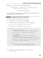
But if I select Show Axis in Thousands, it would look like this (Figure 5-59):
CHAPTER 5 ■ THE STUFF OF LEGEND—CHARTING IN EXCEL
189

Figure 5–59. The Vertical Axis—same values, different look. Note the axis label.
The numbers are trimmed, even though they continue to represent the data in thousands. That is,
the 120 on the axis stands for 120 thousand.
But clicking More Primary Vertical Axis Options… calls up a particularly important dialog box, and
we’ll review some of its options (Figure 5-60):

Figure 5–60. The Format Axis dialog box.
Suppose I wanted to line-chart the hypothetical closing values of the Dow Jones index for one week
(Figure 5-61):
CHAPTER 5 ■ THE STUFF OF LEGEND—CHARTING IN EXCEL
190

Figure 5–61. A week’s worth of stock averages
Excel will yield, for starters, Figure 5-62:

Figure 5–62. Note the values in the Vertical Axis
That minimum value—10200—was chosen by Excel, based on its reading of the chart data. But let

me enter 0 as the lowest chart value, and the chart looks like this (Figure 5-63):
Download From Wow! eBook <www.wowebook.com>
CHAPTER 5 ■ THE STUFF OF LEGEND—CHARTING IN EXCEL
191

Figure 5–63. Same data, different Vertical Axis starting point
And that makes the fluctuation in the closing prices look a lot less dramatic. It’s a classic charting
issue.
Major Unit enables you to change the numeric interval Excel has selected for the Vertical Axis. In
our test-grade chart, the Excel-chosen interval for the grades is 20—0, 20, 40, 60, etc. Enter a Major Unit
of 10 to our grade data, and you get (Figure 5-64):

Figure 5–64. The grades represented in intervals of 10
Note that the Horizontal Gridlines in the plot area are drawn to this interval. Minor Unit lets the
user choose an additional, smaller axis interval that can supplement the major unit. But gridlines
associated with the minor unit don’t appear on the chart by default, a point that takes us to….
The Gridlines option, which enables you to turn on the minor unit gridlines as well. Note in Figure
5-60 the minor unit on our Dow Jones chart is set by default at 4000. If we work with that interval and
select Gridlines: Major and Minor Gridlines, we’ll see (Figure 5-65):
CHAPTER 5 ■ THE STUFF OF LEGEND—CHARTING IN EXCEL
192

Figure 5–65. Major and minor scales: Turning on the minor unit gridlines
(Note: the Gridlines command here is not to be confused with the Gridlines command on the Page
Layout tab, coming in Chapter 9).
And just by way of brief introduction, take note of the Analysis button group. Clicking these options
will, among other things, let you supplement a chart with a trendline drawn atop the chart data, which
tries to portray the trajectory of the data you’re charting (Figure 5-66):

Figure 5–66. Follow the trend: The DJ data accompanied by a trendline

The Analysis group also lets you depict the likely degree of error in a series of values drawn from a
sample, and the like.
CHAPTER 5 ■ THE STUFF OF LEGEND—CHARTING IN EXCEL
193
The Format Tab—Getting Your Objects in Shape
This is probably the easiest Chart tab to figure out, the one whose options can be learned easily through
click-this-button experimentation. The Tab offers a medley of ways to color and slightly reshape any
chart object on which you click, with its options keyed to that object. Thus if you click on a chart plot
area, the Shape Styles drop-down menu (when completely revealed) offers this (Figure 5-67):

Figure 5–67. The Shape of styles to come
Click an option and the plot area takes on the selected color and border effect. The Shape Fill and
Shape Outline buttons are really extensions of Shape Styles, serving up more fill color and border
shaping options. The Shape Effects button makes additional shape embellishments available. Thus click
on a chart plot area, and this Shape Effects potpourri appears (Figure 5-68):

Figure 5–68. Special effects: Shape effects options
Clicking any arrow above reveals still more options.
The WordArt Styles group and its associated Text Fill, Text Outline, and Text Effects options can
reformat any selected text—be it in titles, axes, or legends (Figure 5-69):
CHAPTER 5 ■ THE STUFF OF LEGEND—CHARTING IN EXCEL
194

Figure 5–69. Word Art: Shape effects for text
Note that as indicated earlier, the Format tab has the same Format Selection button on the far left of
its ribbon that you’ll find on the Layout tab.
Sparklines: Mini-Charts with Big Impact
It’s possible that no new feature of Excel 2010 has, uh,—sparked—more advance publicity than
Sparklines, the brainchild of renowned graphics guru Edward Tufte. Sparklines aren’t exactly new,
having been marketed for several years by an array of providers; but once Excel decided to absorb the

product into its interface, it was time to raise an eyebrow or two in the spreadsheet community.
Sparklines are charts of a special sort. Unlike the charts we’ve described to date—objects which
occupy a layer atop the worksheet, as if they were laminated over it—Sparklines are positioned in
worksheet cells, just as any other data are. They have addresses; and thus it’s perfectly reasonable to refer
to the Sparkline in cell I14—something you can’t say about a conventional Excel chart.
And the fact is we’ve already encountered Sparklines—way, way, back in Chapter One, when we first
trotted out that grading worksheet (Figure 5-70):
CHAPTER 5 ■ THE STUFF OF LEGEND—CHARTING IN EXCEL
195

Figure 5–70. Sparklines—mini line charts
Eyes misting with nostalgia? Sentiment aside, those yellow cells contain Sparklines.
Apart from their placement in specific cells, Sparklines differ from conventional Excel charts in
some other important ways:
• They contain no textual information—no titles, axis data, or legends.
• They can only characterize one data series at a time.
• They permit far fewer formatting options.
Thus in view of these limitations, you’re likely ready to ask what’s the up side—that is, why turn to a
Sparkline when a typical Excel chart seems to offer so much more? The answer is that Sparklines can
easily fill a range of cells with their data-capturing magic, allowing for numerous, concise charts keyed
individually to a large span of columns or rows—like our gradebook. As such, they give a quick,
illustrative, graphic read on your data.
So let’s see how Sparklines work. We can return to our set of grades, entered in cells C8:I20. Note
this range includes the class averages as well as the Student name in C9 I warned you about earlier this
chapter (Figure 5-71):
CHAPTER 5 ■ THE STUFF OF LEGEND—CHARTING IN EXCEL
196

Figure 5–71. The grade data, pre-sparkline
To start the Sparkline:

1. Select cells J10:J19. The Sparkline for each student will go here.
2. Click the Insert tab, and then, in the Sparklines button group, click Line. You’ll
see (Figure 5-72 ):

Figure 5–72. The Create Sparkines dialog box
3. In the Data Range field, click D10:H19—the range containing all the student
grades. Here, we’re not worried about that row containing the name Student or
that “Class Average” row—rows 9 and 20, respectively—because we’ve excluded
them from the data range.
CHAPTER 5 ■ THE STUFF OF LEGEND—CHARTING IN EXCEL
197
4. Click OK. The Sparklines in line-chart form should appear in the cells of the
location range—J10:J19, each Sparkline tied to each row of student data.
It’s all pretty easy. One subtle virtue of Sparklines is that you can select a large range of data—say,
daily stock closing prices for an entire year entered across one row, or down one column—and pack it
into one Sparkline, delivering a long-term, global picture of financial activity. Sparklines are also
dynamic—they will continue to register changes in the original source and change accordingly.
And note that because the Sparklines are lodged in cells just like other data, you can select a
Sparkline range, click the Home tab, and click the Fill Color button on the Font button group and color
the cells in which the Sparklines appear. You can then click the Sparkline Tools tab that has magically
appeared above the Design tab (Figure 5-73):

Figure 5–73. The Sparklines Tools tab
and then click the Sparkline Color button on the far right to recolor the Sparklines (Figure 5-74):

Figure 5–74. Where to color Sparklines
You can also modify the lines’ thickness with the Weight option on the same menu.
To emphasize data points in the Sparklines, move left to the Show group (Figure 5-75):

Figure 5–75. The Show group’s buttons, for emphasizing Sparkline data points

CHAPTER 5 ■ THE STUFF OF LEGEND—CHARTING IN EXCEL
198
The Markers button allows you to attach markers to each data point in a line-chart Sparkline (Figure
5-76):

Figure 5–76. Data points on Sparkline line charts
And the other options in that group—High Point, Low Point, Negative Points, First Point, and Last
Point—attach differently-colored markers to each of those points—the highest value in the chart, any
negative values, the very first point in the Sparkline, etc. The Style drop-down menu allows you to select
an overall Spakline motif, coordinating colors for the line and any data markers.
And if you decide you’d rather see your data in columns, you can select the range containing the
Sparklines and click Column on the Sparklines Tools/ Type button group (Figure 5-77):

Figure 5–77. Sparkline chart type options
And boom—there’s your data in columns.
You Win Some, You Lose Some
As the above screen shot attests, you only have three Sparkline chart types to choose from, but in spite of
that modest lineup, the third—Win/Loss—is one that isn’t directly available in the larger conventional
Excel chart roster. The Win/Loss chart is oddly binary—it places a bar above its Horizontal Axis for any
positive number in a cell, and installs a bar below the axis for any negative one. To demonstrate: Say you
begin with this range of numbers (Figure 5-78):
CHAPTER 5 ■ THE STUFF OF LEGEND—CHARTING IN EXCEL
199

Figure 5–78. All or nothing: Positive numbers win, negative numbers lose
Select this range, select the Sparklines Win/Loss chart, and select a one-cell location range to the
right of the range when prompted (though it can really be placed anywhere), and you’ll produce this
(Figure 5-79):

Figure 5–79. In the black: a win-loss chart

Notice there is no magnitude here. All the positive and negative values are recorded equally—
they’re in the same place, either above or below the axis. So why would you use Win/Loss? You could use
it to track the incidence of profits and losses in a business for example, though again, not their exact
values. Win/Loss is often applied to chart wins and losses of sports teams (hence its name); you could
enter a 1 for every team win along a selected range, and a -1 on that same range for every loss. Do this
across a 162-cell range and you could compile a trajectory of the fortunes of a major league baseball
team, by placing a Sparkline in the 163
rd
cell—again, giving the big picture of an entire season. (Note:
Widening a column, or heightening a row, in a Sparkline cell brings about the same kind of aspect ratio
distortion we discussed earlier).
To remove a Sparkline, just right-click it and select Sparklines

Clear Selected Sparklines—it’s
expressed in the plural because you can drag across a range of Sparklines and delete the whole group.
There’s one other important Sparkline set of options, and you’ll find them when you click the Axis
down arrow, in the Sparkline button group (Figure 5-80):

Figure 5–80. Sparkline Axis options
CHAPTER 5 ■ THE STUFF OF LEGEND—CHARTING IN EXCEL
200
You’ll want to know about the Vertical Axis Maximum and Minimum Value Options. The default
Automatic for each Sparkline option means that Excel will decide which numeric intervals will appear on
each Sparkline’s Vertical Axis, after looking at the data. Thus two Sparkline line charts—to return to two
previous examples, one charting a player’s batting averages across his career, the other a series of weight
measurements—will use different intervals on their axes, because the magnitudes are very different. If
you select the same for both Sparklines here, the batting averages and weights will use the same interval
scale—bringing about highly distorted outcomes (Figure 5-81):

Figure 5–81. Heavy hitters: Batting averages charted next to player weights

When they say a player can’t hit his weight, they mean it. The way to make these data readable in
their own terms is to remain with the default Automatic for Each Sparkline, and to set the Custom
Value… option to 0. If you don’t carry out that latter step, the lowest value in each data series is treated
as a de factto zero value, with the other values keyed to it.
As implied above, Custom Value enables you to enter the lowest and highest values of any number
that you’ll allow to appear in a Sparkline. If I enter a lowest allowable value of 1 for the batting average
Sparkline, I’ll see nothing in it—because all the batting averages are fractions, and thus all less than 1.
In Conclusion…
Charting Excel data calls for a two-front approach to the data—understanding how to portray the data in
a lucid and appealing format, and understanding at the same time what you need to do in order to bring
that end about. As we’ve seen, charting options are numerous and variable, depending on the chart
you’ve selected. As always, a bit of practice with real-world charting questions is key. Next up is a closer
look at the data contributing to charts and other Excel capabilities—the world of Excel databases.
Now go out there and cell those charts.
C H A P T E R 6

■ ■ ■

201
Setting the Table: Database
Features of Excel 2010
By now you’ve established a close relationship with the concept of a range—that collection of adjacent
cells occupying a rectangular area on the worksheet (we’ll leave aside any additional nuances I may have
bothered you with earlier). Now, a range can be blank, of course—a collection of adjacent, rectangular-
shaped empty cells is no less a range because of its dearth of data. But when a range is filled with
records—that is, a series of consecutive rows and columns containing related information topped by
headings of the First Name-Last Name-Address variety—you and I might call that assemblage of data a
database. If you were compiling a seating list for a formal event—even if you wrote it out on paper—you
could enter Name and Table Number headings at the top of the page, and pencil in the data accordingly.
Two headings, beneath which you write in the appropriate information; sounds like a database. In Excel,

it could start looking like this (
Figure 6–1):

Figure 6–1. A basic Excel database
That all sounds and looks good to me; but as a terminological matter Excel isn’t always so sure.
Microsoft has had some difficulty making up its mind about exactly what it means by the term database,
though you’re not likely to lose any sleep over the matter, and you shouldn’t. How Microsoft Access
defines “database” doesn’t quite dovetail with the ways it’s been used in Excel, for example—but that
won’t stop us from plunging ahead in any case. I know you like a challenge.
For our purposes, we can go ahead and define a database as a collection of data that occupies
adjacent rows and columns. Each row comprises a record, and each column is a termed a field. Note I’ve
omitted the headings requirement from the definition. Headings are surely a very good thing to find at
the top of a database, but you can still do productive work in a database if they’re not there. What is
CHAPTER 6 ■ SETTING THE TABLE: DATABASE FEATURES OF EXCEL 2010
202
required, however, is that the records in a database be consecutive—because a completely empty row
ropes off the database from any data that may appear on the other side of the blank row. Note,
however—and this is important—that a record need not be complete. As long each record contains at
least one populated field, the database remains in force. Now let’s turn to one classic database option.
Sorting—Sort Of Easy
Think of your little black book—if you still have one—and ask yourself how its contents are arranged.
The probable answer: in alphabetical order, more or less. That’s an equivocal reply, because your book’s
little lettered tabs naturally present themselves in that order, but the names on each page are likely to be
slightly disordered, aren’t they? You’ll post Jones, Jepson, and Jackson to the J’s, but if you’ve entered
them in that sequence, now what? The three aren’t exactly alphabetized, or sorted—and you obviously
won’t erase and rewrite the names each time you make a new entry, in order to ensure a precise listing.
I’d pay big bucks to see you do that.
But spreadsheets (and even word processors) make the sorting process easy, and they can do far
more with the data than anything your black book—or maybe even your Blackberry—can. When I taught
sorting in Excel for a training firm in New York, the manual with which I worked described sorting as an

advanced subject. It isn’t.
The basics—or at least the basic basics—of sorting are most elementary. If you want to sort our old
favorite, the gradebook database:
1. Click anywhere in the column (field) by which you want to sort. Do NOT select
all the cells in that column; just click one cell, as shown in Figure 6–2. (Selecting
the column in its entirety may result in you sorting only that column, and not
the ones on either side of it.)

Figure 6–2. The gradebook with one cell in the test 3 column (field) selected—and ready to sort
2. Click one of the Sort buttons…There’s one—the Sort & Filter button—in the
Editing group in the Home tab (Figure 6–3):
CHAPTER 6 ■ SETTING THE TABLE: DATABASE FEATURES OF EXCEL 2010
203

Figure 6–3. One place to start sorting…
And there are three sorting buttons in the Sort & Filter group on the Data tab (Figure 6–4):

Figure 6–4. …and here’s the other
3. Select the A-Z or Z-A options, representing lowest to highest, or highest to
lowest, respectively. Note the Sort & Filter option in the Editing group requires
you to click a drop-down arrow in order to reach those commands.
That’s it. And to anticipate a common question, the data—all the other adjacent data—are sorted,
too. That means that if you’re sorting these grades by test 3, in Z-A (highest to lowest) order, you’ll get
this (Figure 6–5):
CHAPTER 6 ■ SETTING THE TABLE: DATABASE FEATURES OF EXCEL 2010
204

Figure 6–5. The grades, post-sort
Meaning all the data in all the other adjacent columns remain lined up; nothing is out of whack. We
see Dorothy is still the owner of that 93. Gordon is still jealous. Pretty easy, no? Just click in the desired

column (field), and click A-Z or Z-A.
Using Header Rows
Now there is, however, another big question we need to address. If we sort the above data, why won’t the
very first row be sorted? That is, why isn’t the 3—the number of the test being sorted—treated as just
another test score (a rather low one, too), and thrown to the bottom of the sorted list?
The answer is that sometimes that’s exactly what will happen. But Excel really wants your data to
have a header row—so if it sees a discrepancy between the kind of data in the first row of any field and
the other data in that field, it assumes the first row is a header. And because the last field—Average—is
topped by a text entry, even as the data beneath it are numbers, Excel interprets that data disconnect as
an indicator of a header row; and as a result, it leaves the header row alone. That’s how it works; and it
means in turn that if the Average field had originally been called 6, the first row would have been sorted,
had you clicked in that or any other column.
And the Sort capability also allows you to sort the data by more than one field. Why would you want
to do such a thing? Consider this case: you have a long database of university students, and you want to
sort the records by the Last Name field. Because it’s highly likely that some students will share the same
last name, you would probably want to sort the names further by the First Name field, so that Wilson
Henry is sorted before Wilson Nancy. (If you don’t sort by two fields in cases such as this, the last names
will obviously be sorted together—but the first names will simply remain in their current order). On the
other hand, there’s no reason to sort by a second field if no duplicate data exists in the first. And it also
then follows that if two or more students share the same first and last name, you could sort by a third
field–say, middle initial, or major.
To demonstrate, enter this small database in cells J11:L17 (it should go without saying allthis works
with much larger databases, too) (Figure 6–6):
CHAPTER 6 ■ SETTING THE TABLE: DATABASE FEATURES OF EXCEL 2010
205

Figure 6–6. Note the two Ed Jones entries.
The duplicate data are clear—but I hear some murmuring in the back rows. The eagle-eyed among
you are whispering about the fact that, since all the data—including the headings—are text in nature,
when we go ahead and sort even the header row should be sorted. Very good—it’s all true. So in order to

obviate that problem, let’s move to the next section.
Sorting by More than One Field
To sort by more than one field, click anywhere in the database, and click either the Sort button in the
Data tab, or, in the Home tab, the Sort & Filter button’s down arrow, followed by Custom Sort… (rather
inconsistent, isn’t it). Either way, you’ll be brought to this dialog box (Figure 6–7):

Figure 6–7. The Sort dialog box: Where to sort by multiple columns
Note the check box in the upper right of the dialog box: My data has headers. By checking that box,
you’ll be instructing Excel not to sort the first, or header, row. Then, because we want to sort initially by
Last Name, click the Sort By drop-down arrow and select Last Name (Figure 6–8):
CHAPTER 6 ■ SETTING THE TABLE: DATABASE FEATURES OF EXCEL 2010
206

Figure 6–8. Choosing the fields by which to sort
The Sort On drop-down menu provides you four choices by which to sort—Values, Cell Color, Font
Color, and Cell Icon. Values denotes any data in the cell—and Values here also means text, not just
numbers. The next three options enable you to sort by cells whose appearances may have been changed
by a Conditional Format or even by standard formatting. Thus if you have a range of numerical data, and
you’ve Conditionally Formatted all the numbers in the range greater than 100 red, and all those less than
50 green, you can sort the green cells before the red (Figure 6–9):

Figure 6–9. Sorting by color. It’s done on more than just socks.

CHAPTER 6 ■ SETTING THE TABLE: DATABASE FEATURES OF EXCEL 2010
207
The On top/bottom options are the color-ordering equivalents of A-Z and Z-A. There’s no inherent
ascending or descending color order, after all.
The same idea applies to Cell Icon—if you’ve conditionally formatted certain values to exhibit this
or that icon, they can be sorted first. In our case, though, we’re sorting on values.
Order refers to the direction of the sort—A-Z or Z-A. But there’s another option there, too—Custom

List…. If you have a field whose data consists of days of the week, for example, clicking Custom List and
then clicking the built-in days of the week Custom List (remember that?) lets you work with a sort order
in which Monday can be sorted before Friday, even though the latter comes first alphabetically (and
remember: you can compose your own custom lists, and sort by any of these, too, Figure 6–10).

Figure 6–10. Where to initiate a custom sort
So now we’re ready to sort the database by Last Name—but because we have duplicates in that field,
we want to sort by First Name, too. As a result, we need to click the Add Level button, and select First
Name on the new drop-down arrow alongside that field (Figure 6–11):

Figure 6–11. Sorting by two fields…
CHAPTER 6 ■ SETTING THE TABLE: DATABASE FEATURES OF EXCEL 2010
208
But remember that the database contains two students named Ed Jones, and so we want to sort by
still a third field (and that’s all we have here), in this case, by Major (Figure 6–12):

Figure 6–12. …and now by three
Now that we’ve selected our sort fields, click OK. Here’s what happens (Figure 6–13):

Figure 6–13. Keeping up with Joneses: Note the sort order
Note the two Ed Joneses—sorted together, but with the Poli. Sci. major positioned above Soc.—P
sorted before S. Well done.
There are a few additional Sort dialog box buttons that need to be explained. Delete Level simply
allows you to remove a sort field if you have second thoughts about needing it. Just click the field, select
Delete Level, and it’s gone. Copy Level? Click on a field you’ve already selected to be sorted, click Copy
Level, and that same field appears a second time in the dialog box (Figure 6–14):
CHAPTER 6 ■ SETTING THE TABLE: DATABASE FEATURES OF EXCEL 2010
209

Figure 6–14. Double vision: sorting by the same field twice?

Ok, ok—the question is obvious: Why would you possibly want to copy the same field? And how do
you sort it twice? The answer takes us back to a previous illustration. If you Conditionally Format a range
of values—e.g., cells above 100 red, below 50 green—copying the same field to the Sort dialog box lets
you tell Excel which color in that field gets sorted first, second, etc. Note that some values in the field
might be neither above 100 nor below 50, and thus may have no color. They could be sorted in between
two color priorities, and so you may indeed need to establish a sort order within the same field (there is a
No Color sort option).
The up/down arrows allow you to adjust the order by which fields are sorted. Thus, if you decide
you want the First Name field sorted first, click on First Name and then the up arrow.
Options… delivers a fairly exotic set of choices. First, if you have duplicate names in a field to be
sorted, some of which are lowercase and others capitalized (jones, Jones), sorts the lowercase names
first. Sort left to right allows you to sort by column instead of row. Thus I can sort the columns in the
student database, such that they appear in A-Z sequence: First Name, Last Name, Major.
The AutoFilter: Picking and Choosing Your Data
Sorting data is one of those database have-to-knows, equipped with its variety of options for
reorganizing your information. But sometimes you need to look at only part of the data, based on some
criterion that you’ve established. If you track the sales activity of a team of salespersons, for example,
you may want to see all of Jack and Jill’s transactions, and only their transactions. Or you may want to
generate a list of all the major league players who hit more than 20 home runs last year, or only those
students with test scores under 65. Excel’s AutoFilter does just this kind thing, and it’s even easier than
sorting. It lets you identify which data you want to see with a couple of clicks, and in a couple of seconds.
Let’s try out AutoFilter on our student gradebook. Just click anywhere among the data, click the
Data tab, and click Filter (Figure 6–15):
CHAPTER 6 ■ SETTING THE TABLE: DATABASE FEATURES OF EXCEL 2010
210

Figure 6–15. The Sort & Filter button group
The data look like this (Figure 6–16):

Figure 6–16. Filters in place

You’ll note the handles attaching to the field names (and note AutoFilter assumes the first row is a
header). Now let’s say I want to pull Dorothy’s test results from the data; and while you could object that
Dorothy’s results are already perfectly visible as is, consider that
1. Your list may be hundreds of students long, and Dorothy’s name may not be
quite so evident.
2. Depending on the kind of records you’re keeping, Dorothy’s name could
appear more than once, and in various places down the column, and
3. You may want to print only Dorothy’s data, and hence, need to see only her
information onscreen (Figure 6–16).

Figure 6–17. Filtered data—you may need to see Dorothy’s data alone