beginning excel what if data analysis tool phần 6 ppt
Bạn đang xem bản rút gọn của tài liệu. Xem và tải ngay bản đầy đủ của tài liệu tại đây (743.78 KB, 19 trang )
• The Limits report lists the model’s target cell and the adjustable cells with their respec-
tive values, lower and upper limits, and target values. Use this type of report for problems
that do not contain integer constraints.
To create a report, click one or more report types in the Reports box in the Solver Results
dialog box (see Figure 4-9, shown earlier in the chapter), and then click OK. The corresponding
reports are created on new worksheets in the current workbook, one report per new worksheet.
Interpreting the Answer Report
The Answer report, shown in Figure 4-11, lists the following:
• The target cell’s and adjustable cells’ address, their names if ones were assigned, their
original values before Solver was run, and their final values after Solver was run
• The constraints’ cell addresses, their names if ones were assigned, the cells’ values, the
constraints’ formulas, the constraints’ statuses (Binding, meaning a slack value of 0, or
Not Binding, meaning a nonzero slack value), and the constraints’ slack values
A slack value is the absolute difference in values between the left side and the right side
of the constraint. The left side of the constraint is the constraint cell’s value, and the right
side of the constraint is a specific value or the value of another specified cell. For example, for
a constraint $C$2 >= 2, the slack value is the difference between the value in cell C2 and the
CHAPTER 4 ■ SOLVER74
Figure 4-11. The Solver Answer report (panes split for readability)
5912_c04_final.qxd 10/27/05 10:17 PM Page 74
number 2. For a constraint $A$5 >= $C$2, the slack value is the difference between the values
in cells A5 and C2.
Interpreting the Sensitivity Report
The Sensitivity report (available only for problems that do not contain integer constraints),
shown in Figure 4-12, lists the following:
• The adjustable cells’ addresses and their names if ones were assigned
• The adjustable cells’ final values after Solver was run
• The reduced cost, which is the change in the optimum problem’s outcome per unit
change in the upper or lower bounds of the variable
• The objective coefficient, which measures the relative relationship between the chang-
ing cell and the target cell (for example, if a changing cell’s value is 1.32, and the target
cell’s value is 96, the objective coefficient will be 1.32 divided by 96, or 0.01375)
• The allowable increase and allowable decrease, which indicate how much the problem’s
objective coefficient can change before the optimum solution changes
■Note The limit of 1E+30 appearing in a Solver report is Solver’s way of indicating that any increase is
allowable. Similarly, it displays 1E-30 to indicate that any decrease is allowable.
• The constraints’ cell addresses and their names if ones were assigned
• The constraints’ cells’ final values after Solver was run
• The shadow price, which indicates how much the problem’s objective outcome will
change if you change the right-hand side of the corresponding constraint by one unit,
within the limits given in the Allowable Increase and Allowable Decrease columns
• The right-hand side of the constraint (in the Constraint R.H. Side column), which indi-
cates whether it is a specific value or another cell reference
• The allowable increase and allowable decrease, which indicate how much the con-
straint limit can change and still yield an optimal solution
CHAPTER 4 ■ SOLVER 75
5912_c04_final.qxd 10/27/05 10:17 PM Page 75
Interpreting the Limits Report
The Limits report (available only for problems that do not contain integer constraints) shown
in Figure 4-13, lists the ranges of values over which the maximum and minimum objective val-
ues can be found. The lower limit is the smallest values that the changing cells can contain and
still satisfy the constraints, and the upper limit is the largest values that the changing cells can
contain and still satisfy the constraints.
You can put what you’ve learned about Solver into practice in the previous sections
through the following Try It exercises.
CHAPTER 4 ■ SOLVER76
Figure 4-12. The Solver Sensitivity report
Figure 4-13. The Solver Limits report (panes split for readability)
5912_c04_final.qxd 10/27/05 10:17 PM Page 76
Try It: Use Solver to Solve Math Problems
In this set of exercises, you will use Solver to solve some simple math problems. These exercises
are included in the Excel workbook named Solver Try It Exercises.xls, which is available for
download from the Source Code area of the Apress web site (). The data
for this set of exercises is on the workbook’s Math Problems worksheet, shown in Figure 4-14.
The Math Problems worksheet consists of two parts. The upper part of the worksheet is
used to calculate a cube’s length, width, height, and volume. The lower part of the worksheet
is used to calculate an object’s time, speed, and distance traveled.
Cube Volume Problem
First, use Solver to determine a cube’s volume. Assume a width of at least 4 units; an area of
exactly 80 units; and whole numbers for the length, width, and height.
1. Click Tools
➤ Solver.
2. Click Reset All, and then click OK.
3. Click the Set Target cell box, and then click or type cell B6.
4. Click the Value Of option. In the Value Of box, type 80.
5. Click the By Changing Cells box, and then select cells B3 through B5.
6. Click Add.
7. Click the Cell Reference box, and then click or type cell B4.
8. In the operator box, select =.
9. Click the Constraint box, and then type 4.
10. Click Add.
CHAPTER 4 ■ SOLVER 77
Figure 4-14. The Math Problems worksheet
5912_c04_final.qxd 10/27/05 10:17 PM Page 77
11. Click the Cell Reference box, and then select cells B3 through B5.
12. In the operator box, select Int.
13. Click OK. Your Solver Parameters dialog box should look like Figure 4-15.
14. Click Solve, and then click OK.
Compare your results to Figure 4-16.
Object Velocity Problem
Next, use Solver to determine how long it might take an object to travel 125 kilometers, provided
that the object may not exceed 70 kilometers per hour.
1. Click Tools
➤ Solver.
2. Click Reset All, and then click OK.
3. Click the Set Target cell box, and then click or type cell B12.
4. Click the Value Of option. In the Value Of box, type 125.
CHAPTER 4 ■ SOLVER78
Figure 4-15. The completed Solver Parameters dialog box for the first math problem
Figure 4-16. The Math Problems worksheet after using Solver to determine a cube’s volume,
given several constraints
5912_c04_final.qxd 10/27/05 10:17 PM Page 78
5. Click the By Changing Cells box, and then select cells B10 and B11.
6. Click Add.
7. Click the Cell Reference box, and then click or type cell B11.
8. In the operator box, select =.
9. Click the Constraint box, and then type 70.
10. Click OK. Your Solver Parameters dialog box should look like Figure 4-17.
11. Click Solve, and then click OK.
Compare your results to Figure 4-18.
Try It: Use Solver to Forecast Auction Prices
In this set of exercises, you will use Solver to forecast auction prices for an online auction web
site. The data for this set of exercises is on the Solver Try It Exercises.xls workbook’s Online
Auction worksheet, shown in Figure 4-19.
CHAPTER 4 ■ SOLVER 79
Figure 4-17. The completed Solver Parameters dialog box for the second math problem
Figure 4-18. The Math Problems worksheet after using Solver to determine an object’s time,
speed, and distance traveled
5912_c04_final.qxd 10/27/05 10:17 PM Page 79
The Online Auction worksheet consists of the following:
• Each jewelry item’s description (column A)
• Each jewelry item’s starting auction bid (column B)
• The dollar amount by which each subsequent auction bid for each jewelry item can
be raised (column C)
• The number of auction bids for each jewelry item (column D)
• Each jewelry item’s current bid (column E)
• The number of consecutive days that the bidding period for each jewelry item has
remained open (column F)
• Each jewelry item’s average daily auction bid increase (column G)
Average Daily Bid Increase for One Item
First, use Solver to forecast an average daily auction bid increase of $4.00 for earrings with an
auction length of six days.
1. Click Tools
➤ Solver.
2. Click Reset All, and then click OK.
3. Click the Set Target cell box, and then click or type cell G2.
4. Click the Value Of option. In the Value Of box, type 4.
5. Click the By Changing Cells box. Then click cell D2, press and hold down the Ctrl key,
and click cell F2.
6. Click Add.
7. Click the Cell Reference box, and then click or type cell F2.
8. In the operator box, select =.
9. Click the Constraint box, and then type 6.
10. Click OK. Your Solver Parameters dialog box should look like Figure 4-20.
CHAPTER 4 ■ SOLVER80
Figure 4-19. The Online Auction worksheet
5912_c04_final.qxd 10/27/05 10:17 PM Page 80
11. Click Solve, and then click OK.
Compare your results to Figure 4-21.
Average Daily Auction Bid Increase for All Items
Next, use Solver to forecast an average daily auction bid increase of $12.00 for all current
online auction items, given the following constraints:
• No individual jewelry auction item can have fewer than 3 or more than 12 total bids.
• No individual jewelry auction item can be open for fewer than 3 or more than 10 days.
• The total number of auction bids and the total number of open days for each individual
jewelry auction item must be a whole number.
CHAPTER 4 ■ SOLVER 81
Figure 4-20. The completed Solver Parameters dialog box for the first online auction
problem
Figure 4-21. The Online Auction worksheet after using Solver to determine the earrings’ average
daily auction bid increase, given several constraints
5912_c04_final.qxd 10/27/05 10:17 PM Page 81
■Note This exercise assumes that you have already completed the previous exercise and are starting with
the worksheet values shown in Figure 4-21.
1. Click Tools ➤ Solver.
2. Click Reset All, and then click OK.
3. Click the Set Target cell box, and then click or type cell G7.
4. Click the Value Of option. In the Value Of box, type 12.
5. Click the By Changing Cells box. Then select cells D2 through D6, press and hold
down the Ctrl key, and select cells F2 through F6.
6. Click Add.
7. Click the Cell Reference box, and then select cells D2 through D6.
8. Click the Constraint box, and then type 12.
9. Click Add.
10. Click the Cell Reference box, and then select cells D2 through D6 again.
11. In the operator box, select >=.
12. Click the Constraint box, and then type 3.
13. Click Add.
14. Click the Cell Reference box, and then select cells D2 through D6 again.
15. In the operator box, select Int.
16. Click Add.
17. Click the Cell Reference box, and then select cells F2 through F6.
18. Click the Constraint box, and then type 10.
19. Click Add.
20. Click the Cell Reference box, and then select cells F2 through F6 again.
21. In the operator box, select >=.
22. Click the Constraint box, and then type 3.
23. Click Add.
24. Click the Cell Reference box, and then select cells F2 through F6 again.
25. In the operator box, select Int.
26. Click OK. Your Solver Parameters dialog box should look like Figure 4-22.
CHAPTER 4 ■ SOLVER82
5912_c04_final.qxd 10/27/05 10:17 PM Page 82
27. Click Solve, and then click OK.
Compare your results to Figure 4-23.
Try It: Use Solver to Determine a Home Sales Price
In this exercise, you will use Solver to determine a target home sales price. This exercise’s data
is on the Solver Try It Exercises.xls workbook’s Home Sales worksheet, shown in Figure 4-24.
CHAPTER 4 ■ SOLVER 83
Figure 4-22. The completed Solver Parameters dialog box for the second online auction
problem
Figure 4-23. The Online Auction worksheet after using Solver to determine the average daily
auction bid increase for all current auction items, given several constraints
Figure 4-24. The Home Sales worksheet
5912_c04_final.qxd 10/27/05 10:17 PM Page 83
The Home Sales worksheet consists of the following:
• The total home’s mortgage amount (cell B1)
• The mortgage’s term in months (cell B2)
• The mortgage’s interest rate (cell B3)
• The mortgage’s monthly payment (cell B4)
To keep it simple, assume the mortgage amount is the same as the target home sales price,
and assume the monthly payment covers all aspects of the mortgage, including all taxes and
fees held in escrow.
Use Solver to determine the target home sales price given a payment of no more than
$1,500.00, an interest rate of no more than 5.75%, and a 30-year (360-month) mortgage term.
1. Click Tools
➤ Solver.
2. Click Reset All, and then click OK.
3. Click the Set Target cell box, and then click or type cell B4.
4. Click the Max option.
5. Click the By Changing Cells box, and then select cells B1 through B3.
6. Click Add.
7. Click the Cell Reference box, and then click or type cell B2.
8. In the operator box, select =.
9. Click the Constraint box, and then type 360.
10. Click Add.
11. Click the Cell Reference box, and then click or type cell B3.
12. In the operator box, select =.
13. Click the Constraint box, and then type 0.0575.
14. Click Add.
15. Click the Cell Reference box, and then click or type cell B4.
16. Click the Constraint box, and then type -1500.
17. Click OK. Your Solver Parameters dialog box should look like Figure 4-25.
CHAPTER 4 ■ SOLVER84
5912_c04_final.qxd 10/27/05 10:17 PM Page 84
18. Click Solve, and then click OK.
Compare your results to Figure 4-26.
Try It: Use Solver to Forecast the Weather
In this set of exercises, you will use Solver to forecast the weather. The data for these exercises
is on the Solver Try It Exercises.xls workbook’s Weather worksheet, shown in Figure 4-27.
CHAPTER 4 ■ SOLVER 85
Figure 4-25. The completed Solver Parameters dialog box for the target home sales price
problem
Figure 4-26. The Home Sales worksheet after using Solver to determine the target home sales
price, given several constraints
Figure 4-27. The Weather worksheet (panes split for readability)
5912_c04_final.qxd 10/27/05 10:17 PM Page 85
The Weather worksheet consists of the following:
• The city and state names in which precipitation totals were collected (columns A and B)
• The monthly precipitation totals for each city (columns C through N)
• The yearly precipitation totals for each city (column O)
• The average monthly precipitation for each city (column P)
• The average monthly precipitation for each month (row 27)
Minimum Yearly Precipitation Total for Seattle
First, use Solver to forecast the minimum yearly precipitation total for Seattle. Assume a yearly
precipitation total target of 40 inches; no monthly precipitation total of less than 2 inches; and
no less than 5 inches in January, February, November, or December.
1. Click Tools
➤ Solver.
2. Click Reset All, and then click OK.
3. Click the Set Target cell box, and then click or type cell O24.
4. Click the Value Of option. In the Value Of box, type 40.
5. Click the By Changing Cells box, and then select cells C24 through N24.
6. Click Add.
7. Click the Cell Reference box, and then select cells C24 through N24.
8. In the operator box, select >=.
9. Click the Constraint box, and then type 2.
10. Click Add.
11. Click the Cell Reference box, and then select cells C24 and D24.
12. In the operator box, select >=.
13. Click the Constraint box, and then type 5.
14. Click Add.
15. Click the Cell Reference box, and then select cells M24 and N24.
16. In the operator box, select >=.
17. Click the Constraint box, and then type 5.
18. Click OK. Your Solver Parameters dialog box should look like Figure 4-28.
CHAPTER 4 ■ SOLVER86
5912_c04_final.qxd 10/27/05 10:17 PM Page 86
19. Click Solve, and then click OK.
Compare your results to Figure 4-29.
Average December Precipitation Total for All Cities
Next, use Solver to forecast the average December yearly precipitation total for all cities. Assume
a yearly precipitation combined average of 3 inches, with no monthly precipitation totals of less
than 1 inch or more than 10 inches.
■Note This exercise assumes that you have already completed the previous exercise and are starting with
the worksheet values shown in Figure 4-29.
1. Click Tools ➤ Solver.
2. Click Reset All, and then click OK.
3. Click the Set Target cell box, and then click or type cell N27.
4. Click the Value Of option. In the Value Of box, type 3.
5. Click the By Changing Cells box, and then select cells N2 through N26.
CHAPTER 4 ■ SOLVER 87
Figure 4-28. The completed Solver Parameters dialog box for the first weather problem
Figure 4-29. The Weather worksheet after using Solver to forecast the weather for Seattle, given
several constraints (panes split for readability)
5912_c04_final.qxd 10/27/05 10:17 PM Page 87
6. Click Add.
7. Click the Cell Reference box, and then select cells N2 through N26 again.
8. Click the Constraint box, and then type 10.
9. Click Add.
10. Click the Cell Reference box, and then select cells N2 through N26 again.
11. In the operator box, select >=.
12. Click the Constraint box, and then type 1.
13. Click OK. Your Solver Parameters dialog box should look like Figure 4-30.
14. Click Solve, and then click OK.
Compare your results to Figure 4-31.
Following is a series of seven more involved Solver samples for you to try.
CHAPTER 4 ■ SOLVER88
Figure 4-30. The completed Solver Parameters dialog box for the second weather problem
Figure 4-31. The Weather worksheet after using Solver to forecast the December weather for all
cities, given several constraints (panes split for readability)
5912_c04_final.qxd 10/27/05 10:17 PM Page 88
Try It: Experiment with the Default Solver Samples
Excel includes a series of Solver samples that you can experiment with to learn more about
how to use Solver. These samples can be found in the SOLVSAMP.XLS file. This file is usually
located in the <drive>:\Program Files\Microsoft Office\OFFICE11\SAMPLES folder or the
<drive>:\Program Files\Microsoft Office\Office\SAMPLES folder. This file is installed with
Microsoft Office Excel 2003 when you perform a Complete installation (or a Custom instal-
lation and select Advanced Customization
➤ Microsoft Office ➤ Microsoft Office Excel ➤
Sample Files).
■Note For earlier Office versions, you can usually find the SOLVSAMP.XLS file in the <
drive
>:\Program Files\
Microsoft Office\Office\SAMPLES folder or the <
drive
>:\Office\Examples\Solver folder.
The following sections describe the SOLVSAMP.XLS file’s seven worksheets and provide
exercises for you to experiment with these Solver samples. After you complete each example,
in the Solver Results dialog box, click Restore Original Values, and then click OK to discard the
results and return the cells to their former values. This way, the sample worksheets will not be
changed by your experiments.
Quick Tour
The first worksheet, labeled Quick Tour and partially shown in Figure 4-32, is a marketing
model that shows sales rising from a base figure along with increases in advertising, but with
diminishing returns. For instance, the first $10,000 of advertising in quarter 1 (Q1), in cell B11,
yields about 3,600 incremental units sold (cell B5), but the next $10,000 yields only about 800
units more (cell C5).
CHAPTER 4 ■ SOLVER 89
Figure 4-32. The Quick Tour Solver sample worksheet with its default values
5912_c04_final.qxd 10/27/05 10:17 PM Page 89
As highlighted on the worksheet by a thick cell border, one possible target cell, cell B15,
represents the product profit. The product profit is simply the difference of the gross margin
(cell B8) minus the total costs (cell B13).
For example, in the Quick Tour sample worksheet, you may want to know how much you
could spend on advertising to generate the maximum profit for the year but with a total adver-
tising budget of only $50,000. To figure this out using Solver, do the following:
1. Click Tools
➤ Solver.
2. Click Reset All, and then click OK.
3. Click the Set Target Cell box, and then click cell F15 (Total Product Profit).
4. Click Max.
5. Click the By Changing Cells box, and then select cells B11 through E11 (Advertising).
6. Click Add.
7. Click the Cell Reference box, and then click cell F11 (Total Advertising).
8. Click the Constraint box, and then type 50000.
9. Click OK.
10. Click Solve.
Compare your results to Figure 4-33.
CHAPTER 4 ■ SOLVER90
Figure 4-33. The Quick Tour Solver sample worksheet after using Solver to forecast maximized
profits given an advertising budget limit of $50,000
5912_c04_final.qxd 10/27/05 10:17 PM Page 90
Product Mix
The second worksheet, labeled Product Mix and partially shown in Figure 4-34, portrays a
model of parts for electronic equipment. These parts are in limited supply. You can use Solver
to determine the most profitable mix of electronic equipment to build. However, the profit per
electronic equipment item decreases as more items are built. This is because as each item is
built, you must give equipment sellers volume discounts so that they are inclined to purchase
more items from you at lower and lower prices.
To use Solver to determine the most profitable mix of electronic equipment to build, do
the following:
1. Click Tools
➤ Solver.
2. Click Reset All, and then click OK to clear Solver’s existing settings.
3. Click the Set Target Cell box, and then click cell D18 (Total Profits By Product).
4. Click Max.
5. Click the By Changing Cells box, and then select cells D9 through F9 (Number to Build
for TV Sets, Stereos, and Speakers).
6. Click Add.
7. Click the Cell Reference box, and then select cells C11 through C15 (Number Used).
8. Click the Constraint box, and then select cells B11 through B15 (Inventory).
9. Click Add. This constraint ensures that you will not allocate more parts than are in
your inventory.
CHAPTER 4 ■ SOLVER 91
Figure 4-34. The Product Mix Solver sample worksheet with its default values
5912_c04_final.qxd 10/27/05 10:17 PM Page 91
10. Click the Cell Reference box, and then select cells D9 through F9 (Number to Build for
TV Sets, Stereos, and Speakers).
11. In the operator list, select >=.
12. Click the Constraint box, and then type the number 0.
13. Click OK. This constraint ensures that you will not produce a negative number of elec-
tronic items in any category.
14. Click Options.
15. Clear the Assume Linear Model check box, and then click OK. You need to do this
because the model is nonlinear (due to the factor in cell H15, which shows that profit
per unit diminishes with volume).
16. Click Solve.
Compare your results to Figure 4-35.
Shipping Routes
The third worksheet, labeled Shipping Routes and partially shown in Figure 4-36, is a model
that describes shipping goods from production plants to warehouses. You can use Solver to
minimize the associated shipping costs, while also not exceeding the supply available from
each plant to meet the demand from each warehouse.
CHAPTER 4 ■ SOLVER92
Figure 4-35. The Product Mix Solver sample worksheet after using Solver to forecast the most
profitable mix of electronic equipment to build given several constraints
5912_c04_final.qxd 10/27/05 10:17 PM Page 92