Data Mining Concepts and Techniques phần 6 ppt

362 Chapter 6 Classification and Prediction
cancerous patient is not cancerous) is far greater than that of a false positive (incorrectly
yet conservatively labeling a noncancerous patient as cancerous). In such cases, we can
outweigh one type of error over another by assigning a different cost to each. These
costs may consider the danger to the patient, financial costs of resulting therapies, and
other hospital costs. Similarly, the benefits associated with a true positive decision may
be different than that of a true negative. Up to now, to compute classifier accuracy, we
have assumed equal costs and essentially divided the sum of true positives and true
negatives by the total number of test tuples. Alternatively, we can incorporate costs
and benefits by instead computing the average cost (or benefit) per decision. Other
applications involving cost-benefit analysis include loan application decisions and tar-
get marketing mailouts. For example, the cost of loaning to a defaulter greatly exceeds
that of the lost business incurred by denying a loan to a nondefaulter. Similarly, in an
application that tries to identify households that are likely to respond to mailouts of
certain promotional material, the cost of mailouts to numerous households that do not
respond may outweigh the cost of lost business from not mailing to households that
would have responded. Other costs to consider in the overall analysis include the costs
to collect the data and to develop the classification tool.
“Are there other cases where accuracy may not be appropriate?” In classification prob-
lems, it is commonly assumed that all tuples are uniquely classifiable, that is, that each
training tuple can belong to only one class. Yet, owing to the wide diversity of data
in large databases, it is not always reasonable to assume that all tuples are uniquely
classifiable. Rather, it is more probable to assume that each tuple may belong to more
than one class. How then can the accuracy of classifiers on large databases be mea-
sured? The accuracy measure is not appropriate, because it does not take into account
the possibility of tuples belonging to more than one class.
Rather than returning a class label, it is useful to return a probability class distribu-
tion. Accuracy measures may then use a second guess heuristic, whereby a class pre-
diction is judged as correct if it agrees with the first or second most probable class.
Although this does take into consideration, to some degree, the nonunique classifica-
tion of tuples, it is not a complete solution.

6.12.2 Predictor Error Measures
“How can we measure predictor accuracy?” Let D
T
be a test set of the form (X
1
, y
1
),
(X
2
,y
2
), , (X
d
, y
d
), where the X
i
are the n-dimensional test tuples with associated
known values, y
i
, for a response variable, y, and d is the number of tuples in D
T
. Since
predictors return a continuous value rather than a categorical label, it is difficult to say
exactly whether the predicted value, y

i
, for X
i

is correct. Instead of focusing on whether
y

i
is an “exact” match with y
i
, we instead look at how far off the predicted value is from
the actual known value. Loss functions measure the error between y
i
and the predicted
value, y

i
. The most common loss functions are:
Absolute error : |y
i
−y

i
| (6.59)
Squared error : (y
i
−y

i
)
2
(6.60)
6.13 Evaluating the Accuracy of a Classifier or Predictor 363
Based on the above, the test error (rate), or generalization error, is the average loss

over the test set. Thus, we get the following error rates.
Mean absolute error :
d
∑
i=1
|y
i
−y

i
|
d
(6.61)
Mean squared error :
d
∑
i=1
(y
i
−y

i
)
2
d
(6.62)
The mean squared error exaggerates the presence of outliers, while the mean absolute
error does not. If we were to take the square root of the mean squared error, the result-
ing error measure is called the root mean squared error. This is useful in that it allows
the error measured to be of the same magnitude as the quantity being predicted.

Sometimes, we may want the error to be relative to what it would have been if we
had just predicted
y
, the mean value for y from the training data, D. That is, we can
normalize the total loss by dividing by the total loss incurred from always predicting
the mean. Relative measures of error include:
Relative absolute error :
d
∑
i=1
|y
i
−y

i
|
d
∑
i=1
|y
i
−
y
|
(6.63)
Relative squared error :
d
∑
i=1
(y

i
−y

i
)
2
d
∑
i=1
(y
i
−
y
)
2
(6.64)
where
y
is the mean value of the y
i
’s of the training data, that is
y
=
∑
t
i=1
y
i
d
. We can

take the root of the relative squared error to obtain the root relative squared error so
that the resulting error is of the same magnitude as the quantity predicted.
In practice, the choice of error measure does not greatly affect prediction model
selection.
6.13
Evaluating the Accuracy of a Classifier or Predictor
How can we use the above measures to obtain a reliable estimate of classifier accu-
racy (or predictor accuracy in terms of error)? Holdout, random subsampling, cross-
validation, and the bootstrap are common techniques for assessing accuracy based on
364 Chapter 6 Classification and Prediction
Test set
Training
set
Derive
model
Data
Estimate
accuracy
Figure 6.29 Estimating accuracy with the holdout method.
randomly sampled partitions of the given data. The use of such techniques to estimate
accuracy increases the overall computation time, yet is useful for model selection.
6.13.1 Holdout Method and Random Subsampling
The holdout method is what we have alluded to so far in our discussions about accu-
racy. In this method, the given data are randomly partitioned into two independent
sets, a training set and a test set. Typically, two-thirds of the data are allocated to the
training set, and the remaining one-third is allocated to the test set. The training set is
used to derive the model, whose accuracy is estimated with the test set (Figure 6.29).
The estimate is pessimistic because only a portion of the initial data is used to derive
the model.
Random subsampling is a variation of the holdout method in which the holdout

method is repeated k times. The overall accuracy estimate is taken as the average of the
accuracies obtained from each iteration. (For prediction, we can take the average of the
predictor error rates.)
6.13.2 Cross-validation
In k-fold cross-validation, the initial data are randomly partitioned into k mutually
exclusive subsets or “folds,” D
1
, D
2
, , D
k
, each of approximately equal size. Train-
ing and testing is performed k times. In iteration i, partition D
i
is reserved as the test
set, and the remaining partitions are collectively used to train the model. That is, in
the first iteration, subsets D
2
, , D
k
collectively serve as the training set in order to
obtain a first model, which is tested on D
1
; the second iteration is trained on subsets
D
1
, D
3
, , D
k

and tested on D
2
; and so on. Unlike the holdout and random subsam-
pling methods above, here, each sample is used the same number of times for training
and once for testing. For classification, the accuracy estimate is the overall number of
correct classifications from the k iterations, divided by the total number of tuples in the
initial data. For prediction, the error estimate can be computed as the total loss from
the k iterations, divided by the total number of initial tuples.
6.13 Evaluating the Accuracy of a Classifier or Predictor 365
Leave-one-out is a special case of k-fold cross-validation where k is set to the number
of initial tuples. That is, only one sample is “left out” at a time for the test set. In
stratified cross-validation, the folds are stratified so that the class distribution of the
tuples in each fold is approximately the same as that in the initial data.
In general, stratified 10-fold cross-validation is recommended for estimating accu-
racy (even if computation power allows using more folds) due to its relatively low bias
and variance.
6.13.3 Bootstrap
Unlike the accuracy estimation methods mentioned above, the bootstrap method
samples the given training tuples uniformly with replacement. That is, each time a
tuple is selected, it is equally likely to be selected again and readded to the training set.
For instance, imagine a machine that randomly selects tuples for our training set. In
sampling with replacement, the machine is allowed to select the same tuple more than
once.
There are several bootstrap methods. A commonly used one is the .632 bootstrap,
which works as follows. Suppose we are given a data set of d tuples. The data set is
sampled d times, with replacement, resulting in a bootstrap sample or training set of d
samples. It is very likely that some of the original data tuples will occur more than once
in this sample. The data tuples that did not make it into the training set end up forming
the test set. Suppose we were to try this out several times. As it turns out, on average,
63.2% of the original data tuples will end up in the bootstrap, and the remaining 36.8%

will form the test set (hence, the name, .632 bootstrap.)
“Where does the figure, 63.2%, come from?” Each tuple has a probability of 1/d of
being selected, so the probability of not being chosen is (1−1/d). We have to select d
times, so the probability that a tuple will not be chosen during this whole time is (1−
1/d)
d
. If d is large, the probability approaches e
−1
= 0.368.
14
Thus, 36.8% of tuples
will not be selected for training and thereby end up in the test set, and the remaining
63.2% will form the training set.
We can repeat the sampling procedure k times, where in each iteration, we use the
current test set to obtain an accuracy estimate of the model obtained from the current
bootstrap sample. The overall accuracy of the model is then estimated as
Acc(M) =
k
∑
i=1
(0.632×Acc(M
i
)
test
set
+ 0.368 ×Acc(M
i
)
train set
), (6.65)

where Acc(M
i
)
test
set
is the accuracy of the model obtained with bootstrap sample i
when it is applied to test set i. Acc(M
i
)
train
set
is the accuracy of the model obtained with
bootstrap sample i when it is applied to the original set of data tuples. The bootstrap
method works well with small data sets.
14
e is the base of natural logarithms, that is, e = 2.718.
366 Chapter 6 Classification and Prediction
M
1
Data
M
2
•
•
M
k
Combine
votes
New data
sample

Prediction
Figure 6.30 Increasing model accuracy: Bagging and boosting each generate a set of classification or
prediction models, M
1
, M
2
, , M
k
. Voting strategies are used to combine the predictions
for a given unknown tuple.
6.14
Ensemble Methods—Increasing the Accuracy
In Section 6.3.3, we saw how pruning can be applied to decision tree induction to help
improve the accuracy of the resulting decision trees. Are there general strategies for
improving classifier and predictor accuracy?
The answer is yes. Bagging and boosting are two such techniques (Figure 6.30). They
are examples of ensemble methods, or methods that use a combination of models. Each
combines a series of k learned models (classifiers or predictors), M
1
, M
2
, , M
k
, with
the aim of creating an improved composite model, M∗. Both bagging and boosting can
be used for classification as well as prediction.
6.14.1 Bagging
We first take an intuitive look at how bagging works as a method of increasing accuracy.
For ease of explanation, we will assume at first that our model is a classifier. Suppose
that you are a patient and would like to have a diagnosis made based on your symptoms.

Instead of asking one doctor, you may choose to ask several. If a certain diagnosis occurs
more than any of the others, you may choose this as the final or best diagnosis. That
is, the final diagnosis is made based on a majority vote, where each doctor gets an
equal vote. Now replace each doctor by a classifier, and you have the basic idea behind
bagging. Intuitively, a majority vote made by a large group of doctors may be more
reliable than a majority vote made by a small group.
Given a set, D, of d tuples, bagging works as follows. For iteration i (i = 1, 2, , k), a
training set, D
i
, of d tuples is sampled with replacement from theoriginal set of tuples, D.
Notethattheterm baggingstandsfor bootstrapaggregation. Each trainingset is abootstrap
sample, as described in Section 6.13.3. Because sampling with replacement is used, some
6.14 Ensemble Methods—Increasing the Accuracy 367
Algorithm: Bagging. The bagging algorithm—create an ensemble of models (classifiers or pre-
dictors) for a learning scheme where each model gives an equally-weighted prediction.
Input:
D, a set of d training tuples;
k, the number of models in the ensemble;
a learning scheme (e.g., decision tree algorithm, backpropagation, etc.)
Output: A composite model, M∗.
Method:
(1) for i = 1 to k do // create k models:
(2) create bootstrap sample, D
i
, by sampling D with replacement;
(3) use D
i
to derive a model, M
i
;

(4) endfor
To use the composite model on a tuple, X:
(1) if classification then
(2) let each of the k models classify X and return the majority vote;
(3) if prediction then
(4) let each of the k models predict a value for X and return the average predicted value;
Figure 6.31 Bagging.
of theoriginal tuples of D may not be included inD
i
, whereasothers mayoccur morethan
once. A classifier model, M
i
, is learned for each training set, D
i
. To classify an unknown
tuple, X, each classifier, M
i
, returns its class prediction, which counts as one vote. The
bagged classifier, M∗, counts the votes and assigns the class with the most votes to X.
Bagging can be applied to the prediction of continuous values by taking theaverage value
of each prediction for a given test tuple. The algorithm is summarized in Figure 6.31.
The bagged classifier often has significantly greater accuracy than a single classifier
derived from D, the original training data. It will not be considerably worse and is
more robust to the effects of noisy data. The increased accuracy occurs because the
composite model reduces the variance of the individual classifiers. For prediction, it
was theoretically proven that a bagged predictor will always have improved accuracy
over a single predictor derived from D.
6.14.2 Boosting
We now look at the ensemble method of boosting. As in the previous section, suppose
that as a patient, you have certain symptoms. Instead of consulting one doctor, you

choose to consult several. Suppose you assign weights to the value or worth of each
doctor’s diagnosis, based on the accuracies of previous diagnoses they have made. The
368 Chapter 6 Classification and Prediction
final diagnosis is then a combination of the weighted diagnoses. This is the essence
behind boosting.
In boosting, weights are assigned to each training tuple. A series of k classifiers is
iteratively learned. After a classifier M
i
is learned, the weights are updated to allow the
subsequent classifier, M
i+1
, to “pay more attention” to the training tuples that were mis-
classified by M
i
. The final boosted classifier, M∗, combines the votes of each individual
classifier, where the weight of each classifier’s vote is a function of its accuracy. The
boosting algorithm can be extended for the prediction of continuous values.
Adaboost isapopular boostingalgorithm.Supposewewouldliketoboostthe accuracy
of some learning method. We are given D, a data set of d class-labeled tuples, (X
1
, y
1
),
(X
2
, y
2
), ., (X
d
, y

d
), where y
i
is theclass label of tuple X
i
. Initially, Adaboost assigns each
training tuple an equal weight of 1/d. Generating k classifiers for the ensemble requires
k rounds through the rest of the algorithm. In round i, the tuples from D are sampled to
form a training set, D
i
, of size d. Sampling with replacement is used—the same tuple may
be selected more than once. Each tuple’s chance of being selected is based on its weight.
A classifier model, M
i
, is derived from the training tuples of D
i
. Its error is then calculated
using D
i
as a test set. The weights of the training tuples are then adjusted according to how
they were classified. If a tuple was incorrectly classified, its weight is increased. If a tuple
was correctly classified, its weight is decreased. A tuple’s weight reflects how hard it is to
classify—the higher the weight, the more often it has been misclassified. These weights
will be used to generate the training samples for the classifier of the next round. The basic
idea is that when we build a classifier, we want it to focus more on the misclassified tuples
of the previous round. Some classifiers may be better at classifying some “hard” tuples
than others. In this way, we build a series of classifiers that complement each other. The
algorithm is summarized in Figure 6.32.
Now, let’s look at some of the math that’s involved in the algorithm. To compute
the error rate of model M

i
, we sum the weights of each of the tuples in D
i
that M
i
misclassified. That is,
error(M
i
) =
d
∑
j
w
j
×err(X
j
), (6.66)
where err(X
j
) is the misclassification error of tuple X
j
: If the tuple was misclassified,
then err(X
j
) is 1. Otherwise, it is 0. If the performance of classifier M
i
is so poor that
its error exceeds 0.5, then we abandon it. Instead, we try again by generating a new D
i
training set, from which we derive a new M

i
.
The error rate of M
i
affects how the weights of thetraining tuplesare updated. If a tuple
in round i was correctly classified, its weight is multiplied by error(M
i
)/(1−error(M
i
)).
Once the weights of all of the correctly classified tuples are updated, the weights for all
tuples (including the misclassified ones) are normalized so that their sum remains the
same as it was before. To normalize a weight, we multiply it by the sum of the old weights,
divided by the sum of the new weights. As a result, the weights of misclassified tuples are
increased and the weights of correctly classified tuples are decreased, as described above.
“Once boosting is complete, how is the ensemble of classifiers used to predict the class
label of a tuple, X?” Unlike bagging, where each classifier was assigned an equal vote,
6.14 Ensemble Methods—Increasing the Accuracy 369
Algorithm: Adaboost. A boosting algorithm—create an ensemble of classifiers. Each one gives
a weighted vote.
Input:
D, a set of d class-labeled training tuples;
k, the number of rounds (one classifier is generated per round);
a classification learning scheme.
Output: A composite model.
Method:
(1) initialize the weight of each tuple in D to 1/d;
(2) for i = 1 to k do // for each round:
(3) sample D with replacement according to the tuple weights to obtain D
i

;
(4) use training set D
i
to derive a model, M
i
;
(5) compute error(M
i
), the error rate of M
i
(Equation 6.66)
(6) if error(M
i
) > 0.5 then
(7) reinitialize the weights to 1/d
(8) go back to step 3 and try again;
(9) endif
(10) for each tuple in D
i
that was correctly classified do
(11) multiply the weight of the tuple by error(M
i
)/(1−error(M
i
)); // update weights
(12) normalize the weight of each tuple;
(13) endfor
To use the composite model to classify tuple, X:
(1) initialize weight of each class to 0;
(2) for i = 1 to k do // for each classifier:

(3) w
i
= log
1−error(M
i
)
error(M
i
)
; // weight of the classifier’s vote
(4) c = M
i
(X); // get class prediction for X from M
i
(5) add w
i
to weight for class c
(6) endfor
(7) return the class with the largest weight;
Figure 6.32 Adaboost, a boosting algorithm.
boosting assigns a weight to each classifier’s vote, based on how well the classifier per-
formed. The lower a classifier’s error rate, the more accurate it is, and therefore, the
higher its weight for voting should be. The weight of classifier M
i
’s vote is
log
1−error(M
i
)
error(M

i
)
(6.67)
370 Chapter 6 Classification and Prediction
For each class, c, we sum the weights of each classifier that assigned class c to X. The class
with the highest sum is the “winner” and is returned as the class prediction for tuple X.
“How does boosting compare with bagging?” Because of the way boosting focuses on
the misclassified tuples, it risks overfitting the resulting composite model to such data.
Therefore, sometimes the resulting “boosted” model may be less accurate than a sin-
gle model derived from the same data. Bagging is less susceptible to model overfitting.
While both can significantly improve accuracy in comparison to a single model, boost-
ing tends to achieve greater accuracy.
6.15
Model Selection
Suppose that we have generated two models, M
1
and M
2
(for either classification or
prediction), from our data. We have performed 10-fold cross-validation to obtain a
mean error rate for each. How can we determine which model is best? It may seem
intuitive to select the model with the lowest error rate, however, the mean error rates
are just estimates of error on the true population of future data cases. There can be con-
siderable variance between error rates within any given 10-fold cross-validation exper-
iment. Although the mean error rates obtained for M
1
and M
2
may appear different,
that difference may not be statistically significant. What if any difference between the

two may just be attributed to chance? This section addresses these questions.
6.15.1 Estimating Confidence Intervals
To determine if there is any “real” difference in the mean error rates of two models,
we need to employ a test of statistical significance. In addition, we would like to obtain
some confidence limits for our mean error rates so that we can make statements like
“any observed mean will not vary by +/− two standard errors 95% of the time for future
samples” or “one model is better than the other by a margin of error of +/− 4%.”
What do we need in order to perform the statistical test? Suppose that for each
model, we did 10-fold cross-validation, say, 10 times, each time using a different 10-fold
partitioning of the data. Each partitioning is independently drawn. We can average the
10 error rates obtained each for M
1
and M
2
, respectively, to obtain the mean error
rate for each model. For a given model, the individual error rates calculated in the
cross-validations may be considered as different, independent samples from a proba-
bility distribution. In general, they follow a t distribution with k-1 degrees of freedom
where, here, k = 10. (This distribution looks very similar to a normal, or Gaussian,
distribution even though the functions defining the two are quite different. Both are
unimodal, symmetric, and bell-shaped.) This allows us to do hypothesis testing where
the significance test used is the t-test, or Student’s t-test. Our hypothesis is that the two
models are the same, or in other words, that the difference in mean error rate between
the two is zero. If we can reject this hypothesis (referred to as the null hypothesis), then
we can conclude that the difference between the two models is statistically significant,
in which case we can select the model with the lower error rate.
6.15 Model Selection 371
In data mining practice, we may often employ a single test set, that is, the same test
set can be used for both M
1

and M
2
. In such cases, we do a pairwise comparison of the
two models for each 10-fold cross-validation round. That is, for the ith round of 10-fold
cross-validation, the same cross-validation partitioning is used to obtain an error rate
for M
1
and an error rate for M
2
. Let err(M
1
)
i
(or err(M
2
)
i
) be the error rate of model
M
1
(or M
2
) on round i. The error rates for M
1
are averaged to obtain a mean error
rate for M
1
, denoted
err(M
1

). Similarly, we can obtain err(M
2
). The variance of the
difference between the two models is denoted var(M
1
−M
2
). The t-test computes the
t-statistic with k −1 degrees of freedom for k samples. In our example we have k = 10
since, here, the k samples are our error rates obtained from ten 10-fold cross-validations
for each model. The t-statistic for pairwise comparison is computed as follows:
t =
err(M
1
) −err(M
2
)

var(M
1
−M
2
)/k
, (6.68)
where
var(M
1
−M
2
) =

1
k
k
∑
i=1

err(M
1
)
i
−err(M
2
)
i
−(
err(M
1
) −err(M
2
))

2
. (6.69)
To determine whether M
1
and M
2
are significantly different, we compute t and select
a significance level, sig. In practice, a significance level of 5% or 1% is typically used. We
then consult a table for the t distribution, available in standard textbooks on statistics.

This table is usually shown arranged by degrees of freedom as rows and significance
levels as columns. Suppose we want to ascertain whether the difference between M
1
and
M
2
is significantly different for 95% of the population, that is, sig = 5% or 0.05. We
need to find the t distribution value corresponding to k −1 degrees of freedom (or 9
degrees of freedom for our example) from the table. However, because the t distribution
is symmetric, typically only the upper percentage points of the distribution are shown.
Therefore, we look up the table value for z = sig/2, which in this case is 0.025, where
z is also referred to as a confidence limit. If t > z or t < −z, then our value of t lies in
the rejection region, within the tails of the distribution. This means that we can reject
the null hypothesis that the means of M
1
and M
2
are the same and conclude that there
is a statistically significant difference between the two models. Otherwise, if we cannot
reject the null hypothesis, we then conclude that any difference between M
1
and M
2
can be attributed to chance.
If two test sets are available instead of a single test set, then a nonpaired version of
the t-test is used, where the variance between the means of the two models is estimated
as
var(M
1
−M

2
) =

var(M
1
)
k
1
+
var(M
2
)
k
2
, (6.70)
and k
1
and k
2
are the number of cross-validation samples (in our case, 10-fold cross-
validation rounds) used for M
1
and M
2
, respectively. When consulting the table of t
distribution, the number of degrees of freedom used is taken as the minimum number
of degrees of the two models.
372 Chapter 6 Classification and Prediction
6.15.2 ROC Curves
ROC curves are a useful visual tool for comparing two classification models. The name

ROC stands for Receiver Operating Characteristic. ROC curves come from signal detec-
tion theory that was developed during World War II for the analysis of radar images. An
ROC curve shows the trade-off between the true positive rate or sensitivity (proportion
of positive tuples that are correctly identified) and the false-positive rate (proportion
of negative tuples that are incorrectly identified as positive) for a given model. That
is, given a two-class problem, it allows us to visualize the trade-off between the rate at
which the model can accurately recognize ‘yes’ cases versus the rate at which it mis-
takenly identifies ‘no’ cases as ‘yes’ for different “portions” of the test set. Any increase
in the true positive rate occurs at the cost of an increase in the false-positive rate. The
area under the ROC curve is a measure of the accuracy of the model.
In order to plot an ROC curve for a given classification model, M, the model must
be able to return a probability or ranking for the predicted class of each test tuple.
That is, we need to rank the test tuples in decreasing order, where the one the classifier
thinks is most likely to belong to the positive or ‘yes’ class appears at the top of the list.
Naive Bayesian and backpropagation classifiers are appropriate, whereas others, such
as decision tree classifiers, can easily be modified so as to return a class probability
distribution for each prediction. The vertical axis of an ROC curve represents the true
positive rate. The horizontal axis represents the false-positive rate. An ROC curve for
M is plotted as follows. Starting at the bottom left-hand corner (where the true positive
rate and false-positive rate are both 0), we check the actual class label of the tuple at
the top of the list. If we have a true positive (that is, a positive tuple that was correctly
classified), then on the ROC curve, we move up and plot a point. If, instead, the tuple
really belongs to the ‘no’ class, we have a false positive. On the ROC curve, we move
right and plot a point. This process is repeated for each of the test tuples, each time
moving up on the curve for a true positive or toward the right for a false positive.
Figure 6.33 shows the ROC curves of two classification models. The plot also shows
a diagonal line where for every true positive of such a model, we are just as likely to
encounter a false positive. Thus, the closer the ROC curve of a model is to the diago-
nal line, the less accurate the model. If the model is really good, initially we are more
likely to encounter true positives as we move down the ranked list. Thus, the curve

would move steeply up from zero. Later, as we start to encounter fewer and fewer true
positives, and more and more false positives, the curve cases off and becomes more
horizontal.
To assess the accuracy of a model, we can measure the area under the curve. Several
software packages are able to perform such calculation. The closer the area is to 0.5,
the less accurate the corresponding model is. A model with perfect accuracy will have
an area of 1.0.
6.16 Summary 373
0.0
0.0 0.2 0.4 0.6 0.8 1.0
0.2
0.4
0.6
0.8
1.0
true positive rate
false positive rate
Figure 6.33 The ROC curves of two classification models.
6.16
Summary
Classification and prediction are two forms of data analysis that can be used to extract
models describing important data classes or to predict future data trends. While clas-
sification predicts categorical labels (classes), prediction models continuous-valued
functions.
Preprocessing of the data in preparation for classification and prediction can involve
data cleaning to reduce noise or handle missing values, relevance analysis to remove
irrelevant or redundant attributes, and data transformation, such as generalizing the
data to higher-level concepts or normalizing the data.
Predictive accuracy, computational speed, robustness, scalability, and interpretability
are five criteria for the evaluation of classification and prediction methods.

ID3, C4.5, and CART are greedy algorithms for the induction of decision trees. Each
algorithm uses an attribute selection measure to select the attribute tested for each
nonleaf node in the tree. Pruning algorithms attempt to improve accuracy by remov-
ing tree branches reflecting noise in the data. Early decision tree algorithms typi-
cally assume that the data are memory resident—a limitation to data mining on large
databases. Several scalable algorithms, such as SLIQ, SPRINT, and RainForest, have
been proposed to address this issue.
Naïve Bayesian classification and Bayesian belief networks are based on Bayes, theo-
rem of posterior probability. Unlike naïve Bayesian classification (which assumes class
374 Chapter 6 Classification and Prediction
conditional independence), Bayesian belief networks allow class conditional inde-
pendencies to be defined between subsets of variables.
A rule-based classifier uses a set of IF-THEN rules for classification. Rules can be
extracted from a decision tree. Rules may also be generated directly from training
data using sequential covering algorithms and associative classification algorithms.
Backpropagation is a neural network algorithm for classification that employs a
method of gradient descent. It searches for a set of weights that can model the data
so as to minimize the mean squared distance between the network’s class prediction
and the actual class label of data tuples. Rules may be extracted from trained neural
networks in order to help improve the interpretability of the learned network.
A Support Vector Machine (SVM) is an algorithm for the classification of both linear
and nonlinear data. It transforms the original data in a higher dimension, from where
it can find a hyperplane for separation of the data using essential training tuples called
support vectors.
Associative classification uses association mining techniques that search for frequently
occurring patterns in large databases. The patterns may generate rules, which can be
analyzed for use in classification.
Decision tree classifiers, Bayesian classifiers, classification by backpropagation, sup-
port vector machines, and classification based on association are all examples of eager
learners in that they use training tuples to construct a generalization model and in this

way are ready for classifying new tuples. This contrasts with lazy learners or instance-
based methods of classification, such as nearest-neighbor classifiers and case-based
reasoning classifiers, which store all of the training tuples in pattern space and wait
until presented with a test tuple before performing generalization. Hence, lazy learners
require efficient indexing techniques.
In genetic algorithms, populations of rules “evolve” via operations of crossover and
mutation until all rules within a population satisfy a specified threshold. Rough set
theory can be used to approximately define classes that are not distinguishable based
on the available attributes. Fuzzy set approaches replace “brittle” threshold cutoffs for
continuous-valued attributes with degree of membership functions.
Linear, nonlinear, and generalized linear models of regression can be used for predic-
tion. Many nonlinear problems can be converted to linear problems by performing
transformations on the predictor variables. Unlike decision trees, regression trees and
model trees are used for prediction. In regression trees, each leaf stores a continuous-
valued prediction. In model trees, each leaf holds a regression model.
Stratified k-fold cross-validation is a recommended method for accuracy estimation.
Bagging and boosting methods can be used to increase overall accuracy by learning
and combining a series of individual models. For classifiers, sensitivity, specificity, and
precision are useful alternatives to the accuracy measure, particularly when the main
class of interest is in the minority. There are many measures of predictor error, such as
Exercises 375
the mean squared error, the mean absolute error, the relative squared error, and the
relative absolute error. Significance tests and ROC curves are useful for model
selection.
There have been numerous comparisons of the different classification and prediction
methods, and the matter remains a research topic. No single method has been found
to be superior over all others for all data sets. Issues such as accuracy, training time,
robustness, interpretability, and scalability must be considered and can involve trade-
offs, further complicating the quest for an overall superior method. Empirical studies
show that the accuracies of many algorithms are sufficiently similar that their differ-

ences are statistically insignificant, while training times may differ substantially. For
classification, most neural network and statistical methods involving splines tend to
be more computationally intensive than most decision tree methods.
Exercises
6.1 Briefly outline the major steps of decision tree classification.
6.2 Why is tree pruning useful in decision tree induction? What is a drawback of using a
separate set of tuples to evaluate pruning?
6.3 Given a decision tree, you have the option of (a) converting the decision tree to rules
and then pruning the resulting rules, or (b) pruning the decision tree and then con-
verting the pruned tree to rules. What advantage does (a) have over (b)?
6.4 It is important to calculate the worst-case computational complexity of the decision
tree algorithm. Given data set D, the number of attributes n, and the number of
training tuples |D|, show that the computational cost of growing a tree is at most
n×|D|×log(|D|).
6.5 Why is naïve Bayesian classification called “naïve”? Briefly outline the major ideas of
naïve Bayesian classification.
6.6 Given a 5 GB data set with 50 attributes (each containing 100 distinct values) and
512 MB of main memory in your laptop, outline an efficient method that constructs
decision trees in such large data sets. Justify your answer by rough calculation of your
main memory usage.
6.7 RainForest is an interesting scalable algorithm for decision tree induction. Develop a
scalable naive Bayesian classification algorithm that requires just a single scan of the
entire data set for most databases. Discuss whether such an algorithm can be refined
to incorporate boosting to further enhance its classification accuracy.
6.8 Compare the advantages and disadvantages of eager classification (e.g., decision tree,
Bayesian, neural network) versus lazy classification (e.g., k-nearest neighbor, case-
based reasoning).
6.9 Design an efficient method that performs effective naïve Bayesian classification over
an infinite data stream (i.e., you can scan the data stream only once). If we wanted to
376 Chapter 6 Classification and Prediction

discover the evolution of such classification schemes (e.g., comparing the classification
scheme at this moment with earlier schemes, such as one from a week ago), what
modified design would you suggest?
6.10 What is associative classification? Why is associative classification able to achieve higher
classification accuracy than a classical decision tree method? Explain how associative
classification can be used for text document classification.
6.11 The following table consists of training data from an employee database. The data
have been generalized. For example, “31 35” for age represents the age range of 31
to 35. For a given row entry, count represents the number of data tuples having the
values for department, status, age, and salary given in that row.
department status age salary count
sales senior 31 35 46K 50K 30
sales junior 26 30 26K 30K 40
sales junior 31 35 31K 35K 40
systems junior 21 25 46K 50K 20
systems senior 31 35 66K 70K 5
systems junior 26 30 46K 50K 3
systems senior 41 45 66K 70K 3
marketing senior 36 40 46K 50K 10
marketing junior 31 35 41K 45K 4
secretary senior 46 50 36K 40K 4
secretary junior 26 30 26K 30K 6
Let status be the class label attribute.
(a) How would you modify the basic decision tree algorithm to take into considera-
tion the count of each generalized data tuple (i.e., of each row entry)?
(b) Use your algorithm to construct a decision tree from the given data.
(c) Given a data tuple having the values “systems,” “26 30,” and “46–50K” for the
attributes department, age, and salary, respectively, what would a naive Bayesian
classification of the status for the tuple be?
(d) Design a multilayer feed-forward neural network for the given data. Label the

nodes in the input and output layers.
(e) Using the multilayer feed-forward neural network obtained above, show the weight
values after one iteration of the backpropagation algorithm, given the training
instance “(sales, senior,31 35, 46K 50K).” Indicate your initial weight values and
biases, and the learning rate used.
6.12 The support vector machine (SVM) is a highly accurate classification method. However,
SVM classifiers suffer from slow processing when training with a large set of data
Exercises 377
tuples. Discuss how to overcome this difficulty and develop a scalable SVM algorithm
for efficient SVM classification in large datasets.
6.13 Write an algorithm for k-nearest-neighbor classification given k and n, the number of
attributes describing each tuple.
6.14 The following table shows the midterm and final exam grades obtained for students
in a database course.
x y
Midterm exam Final exam
72 84
50 63
81 77
74 78
94 90
86 75
59 49
83 79
65 77
33 52
88 74
81 90
(a) Plot the data. Do x and y seem to have a linear relationship?
(b) Use the method of least squares to find an equation for the prediction of a student’s

final exam grade based on the student’s midterm grade in the course.
(c) Predict the final exam grade of a student who received an 86 on the midterm
exam.
6.15 Some nonlinear regression models can be converted to linear models by applying trans-
formations to the predictor variables. Show how the nonlinear regression equation
y = αX
β
can be converted to a linear regression equation solvable by the method of
least squares.
6.16 What is boosting? State why it may improve the accuracy of decision tree induction.
6.17 Showthataccuracyisafunctionofsensitivityandspecificity,thatis,proveEquation(6.58).
6.18 Suppose that we would like to select between two prediction models, M
1
and M
2
. We
have performed 10 rounds of 10-fold cross-validation on each model, where the same
data partitioning in round i is used for both M
1
and M
2
. The error rates obtained for
M
1
are 30.5, 32.2, 20.7, 20.6, 31.0, 41.0, 27.7, 26.0, 21.5, 26.0. The error rates for M
2
are 22.4, 14.5, 22.4, 19.6, 20.7, 20.4, 22.1, 19.4, 16.2, 35.0. Comment on whether one
model is significantly better than the other considering a significance level of 1%.
378 Chapter 6 Classification and Prediction
6.19 It is difficult to assess classification accuracy when individual data objects may belong

to more than one class at a time. In such cases, comment on what criteria you would
use to compare different classifiers modeled after the same data.
Bibliographic Notes
Classification from machine learning, statistics, and pattern recognition perspectives
has been described in many books, such as Weiss and Kulikowski [WK91], Michie,
Spiegelhalter,and Taylor [MST94], Russel and Norvig [RN95], Langley [Lan96], Mitchell
[Mit97], Hastie, Tibshirani, and Friedman [HTF01], Duda, Hart, and Stork [DHS01],
Alpaydin [Alp04], Tan, Steinbach, and Kumar [TSK05], and Witten and Frank [WF05].
Many of these books describe each of the basic methods of classification discussed in this
chapter,as well as practical techniques for the evaluation of classifier performance. Edited
collections containing seminal articles on machine learning can be found in Michalski,
Carbonell, and Mitchell [MCM83,MCM86], Kodratoff and Michalski [KM90], Shavlik
and Dietterich [SD90], and Michalski and Tecuci [MT94]. For a presentation of machine
learning with respect to data mining applications, see Michalski, Bratko, and Kubat
[MBK98].
The C4.5 algorithm is described in a book by Quinlan [Qui93]. The CART system is
detailed in Classification and Regression Trees by Breiman, Friedman, Olshen, and Stone
[BFOS84]. Both books give an excellent presentation of many of the issues regarding
decision tree induction. C4.5 has a commercial successor, known as C5.0, which can be
found at www.rulequest.com. ID3, a predecessor of C4.5, is detailed in Quinlan [Qui86].
It expands on pioneering work on concept learning systems, described by Hunt, Marin,
and Stone [HMS66]. Other algorithms for decision tree induction include FACT (Loh
and Vanichsetakul [LV88]), QUEST (Loh and Shih [LS97]), PUBLIC (Rastogi and Shim
[RS98]), and CHAID (Kass [Kas80] and Magidson [Mag94]). INFERULE (Uthurusamy,
Fayyad, and Spangler [UFS91]) learns decision trees from inconclusive data, where prob-
abilistic rather than categorical classification rules are obtained. KATE (Manago and
Kodratoff [MK91]) learns decision trees from complex structured data. Incremental ver-
sions of ID3 include ID4 (Schlimmer and Fisher [SF86a]) and ID5 (Utgoff [Utg88]), the
latter of which is extended in Utgoff, Berkman, and Clouse [UBC97]. An incremental
version of CART is described in Crawford [Cra89]. BOAT (Gehrke, Ganti, Ramakrish-

nan, and Loh [GGRL99]), a decision tree algorithm that addresses the scalabilty issue
in data mining, is also incremental. Other decision tree algorithms that address scalabil-
ity include SLIQ (Mehta, Agrawal, and Rissanen [MAR96]), SPRINT (Shafer, Agrawal,
and Mehta [SAM96]), RainForest (Gehrke, Ramakrishnan, and Ganti [GRG98]), and
earlier approaches, such as Catlet [Cat91], and Chan and Stolfo [CS93a, CS93b]. The
integration of attribution-oriented induction with decision tree induction is proposed
in Kamber, Winstone, Gong, et al. [KWG
+
97]. For a comprehensive survey of many
salient issues relating to decision tree induction, such as attribute selection and pruning,
see Murthy [Mur98].
Bibliographic Notes 379
For a detailed discussion on attribute selection measures, see Kononenko and Hong
[KH97]. Information gain was proposed by Quinlan [Qui86] and is based on pioneering
work on information theory by Shannon and Weaver [SW49]. The gain ratio, proposed
as an extension to information gain, is described as part of C4.5 [Qui93]. The Gini index
was proposed for CART [BFOS84]. The G-statistic, based on information theory, is given
in Sokal and Rohlf [SR81]. Comparisons of attribute selection measures include Bun-
tine and Niblett [BN92], Fayyad and Irani [FI92], Kononenko [Kon95], Loh and Shih
[LS97], and Shih [Shi99]. Fayyad and Irani [FI92] show limitations of impurity-based
measures such as information gain and Gini index. They propose a class of attribute
selection measures called C-SEP (Class SEParation), which outperform impurity-based
measures in certain cases. Kononenko [Kon95] notes that attribute selection measures
based on the minimum description length principle have the least bias toward multival-
ued attributes. Martin and Hirschberg [MH95] proved that the time complexity of deci-
sion tree induction increases exponentially with respect to tree height in the worst case,
and under fairly general conditions in the average case. Fayad and Irani [FI90] found
that shallow decision trees tend to have many leaves and higher error rates for a large
variety of domains. Attribute (or feature) construction is described in Liu and Motoda
[LM98, Le98]. Examples of systems with attribute construction include BACON by Lan-

gley, Simon, Bradshaw, and Zytkow [LSBZ87], Stagger by Schlimmer [Sch86], FRINGE
by Pagallo [Pag89], and AQ17-DCI by Bloedorn and Michalski [BM98].
There are numerous algorithms for decision tree pruning, including cost complex-
ity pruning (Breiman, Friedman, Olshen, and Stone [BFOS84]), reduced error prun-
ing (Quinlan [Qui87]), and pessimistic pruning (Quinlan [Qui86]). PUBLIC (Rastogi
and Shim [RS98]) integrates decision tree construction with tree pruning. MDL-based
pruning methods can be found in Quinlan and Rivest [QR89], Mehta, Agrawal, and
Rissanen [MRA95], and Rastogi and Shim [RS98]. Other methods include Niblett and
Bratko [NB86], and Hosking, Pednault, and Sudan [HPS97]. For an empirical compar-
ison of pruning methods, see Mingers [Min89] and Malerba, Floriana, and Semeraro
[MFS95]. For a survey on simplifying decision trees, see Breslow and Aha [BA97].
There are several examples of rule-based classifiers. These include AQ15 (Hong,
Mozetic, and Michalski [HMM86]), CN2 (Clark and Niblett [CN89]), ITRULE (Smyth
and Goodman [SG92]), RISE (Domingos [Dom94]), IREP (Furnkranz and Widmer
[FW94]), RIPPER (Cohen [Coh95]), FOIL (Quinlan and Cameron-Jones [Qui90,
QCJ93]), and Swap-1 (Weiss and Indurkhya [WI98]). For the extraction of rules from
decision trees, see Quinlan [Qui87, Qui93]. Rule refinement strategies that identify the
most interesting rules among a given rule set can be found in Major and Mangano
[MM95].
Thorough presentations of Bayesian classification can be found in Duda, Hart, and
Stork [DHS01], Weiss and Kulikowski [WK91], and Mitchell [Mit97]. For an anal-
ysis of the predictive power of naïve Bayesian classifiers when the class conditional
independence assumption is violated, see Domingos and Pazzani [DP96]. Experiments
with kernel density estimation for continuous-valued attributes, rather than Gaussian
estimation, have been reported for naïve Bayesian classifiers in John [Joh97]. For an
introduction to Bayesian belief networks, see Heckerman [Hec96]. For a thorough
380 Chapter 6 Classification and Prediction
presentation of probabilistic networks, see Pearl [Pea88]. Solutions for learning the
belief network structure from training data given observable variables are proposed in
Cooper and Herskovits [CH92], Buntine [Bun94], and Heckerman, Geiger, and Chick-

ering [HGC95]. Algorithms for inference on belief networks can be found in Russell
and Norvig [RN95] and Jensen [Jen96]. The method of gradient descent, described in
Section 6.4.4 for training Bayesian belief networks, is given in Russell, Binder, Koller,
and Kanazawa [RBKK95]. The example given in Figure 6.11 is adapted from Russell
et al. [RBKK95]. Alternative strategies for learning belief networks with hidden vari-
ables include application of Dempster, Laird, and Rubin’s [DLR77] EM (Expectation
Maximization) algorithm (Lauritzen [Lau95]) and methods based on the minimum
description length principle (Lam [Lam98]). Cooper [Coo90] showed that the general
problem of inference in unconstrained belief networks is NP-hard. Limitations of belief
networks, such as their large computational complexity (Laskey and Mahoney [LM97]),
have prompted the exploration of hierarchical and composable Bayesian models (Pfef-
fer, Koller, Milch, and Takusagawa [PKMT99] and Xiang, Olesen, and Jensen [XOJ00]).
These follow an object-oriented approach to knowledge representation.
The perceptron is a simple neural network, proposed in 1958 by Rosenblatt [Ros58],
which became a landmark in early machine learning history. Its input units are ran-
domly connected to a single layer of output linear threshold units. In 1969, Minsky
and Papert [MP69] showed that perceptrons are incapable of learning concepts that
are linearly inseparable. This limitation, as well as limitations on hardware at the time,
dampened enthusiasm for research in computational neuronal modeling for nearly 20
years. Renewed interest was sparked following presentation of the backpropagation
algorithm in 1986 by Rumelhart, Hinton, and Williams [RHW86], as this algorithm
can learn concepts that are linearly inseparable. Since then, many variations for back-
propagation have been proposed, involving, for example, alternative error functions
(Hanson and Burr [HB88]), dynamic adjustment of the network topology (Me´zard
and Nadal [MN89], Fahlman and Lebiere [FL90], Le Cun, Denker, and Solla [LDS90],
and Harp, Samad, and Guha [HSG90] ), and dynamic adjustment of the learning rate
and momentum parameters (Jacobs [Jac88]). Other variations are discussed in Chauvin
and Rumelhart [CR95]. Books on neural networks include Rumelhart and McClelland
[RM86], Hecht-Nielsen [HN90], Hertz, Krogh, and Palmer [HKP91], Bishop [Bis95],
Ripley [Rip96], and Haykin [Hay99]. Many books on machine learning, such as [Mit97,

RN95], also contain good explanations of the backpropagation algorithm. There are
several techniques for extracting rules from neural networks, such as [SN88, Gal93,
TS93, Avn95, LSL95, CS96b, LGT97]. The method of rule extraction described in Sec-
tion 6.6.4 is based on Lu, Setiono, and Liu [LSL95]. Critiques of techniques for rule
extraction from neural networks can be found in Craven and Shavlik [CS97]. Roy
[Roy00] proposes that the theoretical foundations of neural networks are flawed with
respect to assumptions made regarding how connectionist learning models the brain.
An extensive survey of applications of neural networks in industry, business, and sci-
ence is provided in Widrow, Rumelhart, and Lehr [WRL94].
Support Vector Machines (SVMs) grew out of early work by Vapnik and Chervonenkis
on statistical learning theory [VC71]. The first paper on SVMs was presented by Boser,
Bibliographic Notes 381
Guyon, and Vapnik [BGV92]. More detailed accounts can be found in books by Vapnik
[Vap95, Vap98]. Good startingpoints includethe tutorialon SVMsby Burges [Bur98]and
textbook coverage by Kecman [Kec01]. For methods for solving optimization problems,
see Fletcher [Fle87] and Nocedal and Wright [NW99]. These references give additional
details alluded to as “fancy math tricks” in our text,such as transformation of the problem
to a Lagrangian formulation and subsequent solving using Karush-Kuhn-Tucker (KKT)
conditions. For the application of SVMs to regression, see Schlkopf, Bartlett, Smola, and
Williamson [SBSW99], and Drucker, Burges, Kaufman, Smola, and Vapnik [DBK
+
97].
Approaches to SVM for large data include the sequential minimal optimization algo-
rithm by Platt [Pla98], decomposition approaches such as in Osuna, Freund, and Girosi
[OFG97], and CB-SVM, a microclustering-based SVM algorithm for large data sets, by
Yu, Yang, and Han [YYH03].
Many algorithms have been proposed that adapt association rule mining to the task
of classification. The CBA algorithm for associative classification was proposed by Liu,
Hsu, and Ma [LHM98]. A classifier, using emerging patterns, was proposed by Dong
and Li [DL99] and Li, Dong, and Ramamohanarao [LDR00]. CMAR (Classification

based on Multiple Association Rules) was presented in Li, Han, and Pei [LHP01]. CPAR
(Classification based on Predictive Association Rules) was proposed in Yin and Han
[YH03b]. Cong, Tan, Tung, and Xu proposed a method for mining top-k covering rule
groups for classifying gene expression data with high accuracy [CTTX05]. Lent, Swami,
and Widom [LSW97] proposed the ARCS system, which was described in Section 5.3
on mining multidimensional association rules. It combines ideas from association rule
mining, clustering, and image processing, and applies them to classification. Meretakis
and Wüthrich [MW99] proposed to construct a naïve Bayesian classifier by mining
long itemsets.
Nearest-neighbor classifiers were introduced in 1951 by Fix and Hodges [FH51].
A comprehensive collection of articles on nearest-neighbor classification can be found
in Dasarathy [Das91]. Additional references can be found in many texts on classifica-
tion, such as Duda et al. [DHS01] and James [Jam85], as well as articles by Cover and
Hart [CH67] and Fukunaga and Hummels [FH87]. Their integration with attribute-
weighting and the pruning of noisy instances is described in Aha [Aha92]. The use of
search trees to improve nearest-neighbor classification time is detailed in Friedman,
Bentley, and Finkel [FBF77]. The partial distance method was proposed by researchers
in vector quantization and compression. It is outlined in Gersho and Gray [GG92].
The editing method for removing “useless” training tuples was first proposed by Hart
[Har68]. The computational complexity of nearest-neighbor classifiers is described in
Preparata and Shamos [PS85]. References on case-based reasoning (CBR) include the
texts Riesbeck and Schank [RS89] and Kolodner [Kol93], as well as Leake [Lea96] and
Aamodt and Plazas [AP94]. For a list of business applications, see Allen [All94]. Exam-
ples in medicine include CASEY by Koton [Kot88] and PROTOS by Bareiss, Porter, and
Weir [BPW88], while Rissland and Ashley [RA87] is an example of CBR for law. CBR
is available in several commercial software products. For texts on genetic algorithms, see
Goldberg [Gol89], Michalewicz [Mic92], and Mitchell [Mit96]. Rough sets were
introduced in Pawlak [Paw91]. Concise summaries of rough set theory in data
382 Chapter 6 Classification and Prediction
mining include Ziarko [Zia91], and Cios, Pedrycz, and Swiniarski [CPS98]. Rough

sets have been used for feature reduction and expert system design in many applica-
tions, including Ziarko [Zia91], Lenarcik and Piasta [LP97], and Swiniarski [Swi98].
Algorithms to reduce the computation intensity in finding reducts have been proposed
in Skowron and Rauszer [SR92]. Fuzzy set theory was proposed by Zadeh in [Zad65,
Zad83]. Additional descriptions can be found in [YZ94, Kec01].
Many good textbooks cover the techniques of regression. Examples include James
[Jam85], Dobson [Dob01], Johnson and Wichern [JW02], Devore [Dev95], Hogg and
Craig [HC95], Neter, Kutner, Nachtsheim, and Wasserman [NKNW96], and Agresti
[Agr96]. The book by Press, Teukolsky, Vetterling, and Flannery [PTVF96] and accom-
panying source code contain many statistical procedures, such as the method of least
squares for both linear and multiple regression. Recent nonlinear regression models
include projection pursuit and MARS (Friedman [Fri91]). Log-linear models are also
known in the computer science literature as multiplicative models. For log-linear mod-
els from a computer science perspective, see Pearl [Pea88]. Regression trees (Breiman,
Friedman, Olshen, and Stone [BFOS84]) are often comparable in performance with
other regression methods, particularly when there exist many higher-order dependen-
cies among the predictor variables. For model trees, see Quinlan [Qui92].
Methods for data cleaning and data transformation are discussed in Kennedy, Lee,
Van Roy, et al. [KLV
+
98], Weiss and Indurkhya [WI98], Pyle [Pyl99], and Chapter 2
of this book. Issues involved in estimating classifier accuracy are described in Weiss
and Kulikowski [WK91] and Witten and Frank [WF05]. The use of stratified 10-fold
cross-validation for estimating classifier accuracy is recommended over the holdout,
cross-validation, leave-one-out (Stone [Sto74]) and bootstrapping (Efron and Tibshi-
rani [ET93]) methods, based on a theoretical and empirical study by Kohavi [Koh95].
Bagging is proposed in Breiman [Bre96]. The boosting technique of Freund and
Schapire [FS97] has been applied to several different classifiers, including decision tree
induction (Quinlan [Qui96]) and naive Bayesian classification (Elkan [Elk97]). Sensi-
tivity, specificity, and precision are discussed in Frakes and Baeza-Yates [FBY92]. For

ROC analysis, see Egan [Ega75] and Swets [Swe88].
The University of California at Irvine (UCI) maintains a Machine Learning Repos-
itory of data sets for the development and testing of classification algorithms. It also
maintains a Knowledge Discovery in Databases (KDD) Archive, an online repository of
large data sets that encompasses a wide variety of data types, analysis tasks, and appli-
cation areas. For information on these two repositories, see www.ics.uci.edu/~mlearn/
MLRepository.html and .
No classification method is superior over all others for all data types and domains.
Empirical comparisons of classification methods include [Qui88, SMT91, BCP93,
CM94, MST94, BU95], and [LLS00].
7
Cluster Analysis
Imagine that you are given a set of data objects for analysis where, unlike in classification, the class
label of each object is not known. This is quite common in large databases, because
assigning class labels to a large number of objects can be a very costly process. Clustering
is the process of grouping the data into classes or clusters, so that objects within a clus-
ter have high similarity in comparison to one another but are very dissimilar to objects
in other clusters. Dissimilarities are assessed based on the attribute values describing the
objects. Often, distance measures are used. Clustering has its roots in many areas, includ-
ing data mining, statistics, biology, and machine learning.
In this chapter, we study the requirements of clustering methods for large amounts of
data. We explain how to compute dissimilarities between objects represented by various
attribute or variable types. We examine several clustering techniques, organized into the
following categories: partitioning methods, hierarchical methods, density-based methods,
grid-based methods, model-based methods, methods for high-dimensional data (such as
frequent pattern–based methods), and constraint-based clustering. Clustering can also be
used for outlier detection, which forms the final topic of this chapter.
7.1
What Is Cluster Analysis?
The process of grouping a set of physical or abstract objects into classes of similar objects

is called clustering. A cluster is a collection of data objects that are similar to one another
within the same cluster and are dissimilar to the objects in other clusters. A cluster of data
objects can be treated collectively as one group and so may be considered as a form of data
compression. Although classification is an effective means for distinguishing groups or
classesof objects, itrequiresthe often costlycollectionand labeling of a large setof training
tuples or patterns, which the classifier uses to model each group. It is often more desirable
to proceedin thereverse direction: First partition the set ofdata into groups based on data
similarity (e.g., using clustering), and then assign labels to the relatively small number of
groups. Additional advantages of such a clustering-based process are that it is adaptable
to changes and helps single out useful features that distinguish different groups.
383
384 Chapter 7 Cluster Analysis
Cluster analysis is an important human activity. Early in childhood, we learn how
to distinguish between cats and dogs, or between animals and plants, by continuously
improving subconscious clustering schemes. By automated clustering, we can identify
dense and sparse regions in object space and, therefore, discover overall distribution pat-
terns and interesting correlations among data attributes. Cluster analysis has been widely
used in numerous applications, including market research, pattern recognition, data
analysis, and image processing. In business, clustering can help marketers discover dis-
tinct groups in their customer bases and characterize customer groups based on
purchasing patterns. In biology, it can be used to derive plant and animal taxonomies,
categorize genes with similar functionality, and gain insight into structures inherent in
populations. Clustering may also help in the identification of areas of similar land use
in an earth observation database and in the identification of groups of houses in a city
according to house type, value, and geographic location, as well as the identification of
groups of automobile insurance policy holders with a high average claim cost. It can also
be used to help classify documents on the Web for information discovery.
Clustering is also called data segmentation in some applications because clustering
partitions large data sets into groups according to their similarity. Clustering can also be
used for outlier detection, where outliers (values that are “far away” from any cluster)

may be more interesting than common cases. Applications of outlier detection include
the detection of credit card fraud and the monitoring of criminal activities in electronic
commerce. For example, exceptional cases incredit card transactions, such as very expen-
sive and frequent purchases, may be of interest as possible fraudulent activity. As a data
mining function, cluster analysis can be used as a stand-alone tool to gain insight into
the distribution of data, to observe the characteristics of each cluster, and to focus on a
particular set of clusters for further analysis. Alternatively, it may serve as a preprocessing
step for other algorithms, such as characterization, attribute subset selection, and clas-
sification, which would then operate on the detected clusters and the selected attributes
or features.
Data clustering is under vigorous development. Contributing areas of research include
data mining, statistics, machine learning, spatial database technology, biology, and mar-
keting. Owing to the huge amounts of data collected in databases, cluster analysis has
recently become a highly active topic in data mining research.
As a branch of statistics, cluster analysis has been extensively studied for many years,
focusing mainly on distance-based cluster analysis. Cluster analysis tools based on
k-means, k-medoids, and several other methods have also been built into many statistical
analysis software packages or systems, such as S-Plus, SPSS, and SAS. In machine learn-
ing, clustering is an example of unsupervised learning. Unlike classification, clustering
and unsupervised learning do not rely on predefined classes and class-labeled training
examples. For this reason, clustering is a form of learning by observation, rather than
learning by examples. In data mining, efforts have focused on finding methods for effi-
cient and effective cluster analysis in large databases. Active themes of research focus on
the scalability of clustering methods, the effectiveness of methods for clustering complex
shapes and types of data, high-dimensional clustering techniques, and methods for clus-
tering mixed numerical and categorical data in large databases.
7.1 What Is Cluster Analysis? 385
Clustering is a challenging field of research in which its potential applications pose
their own special requirements. The following are typical requirements of clustering in
data mining:

Scalability: Many clustering algorithms work well on small data sets containing fewer
than several hundred data objects; however, a large database may contain millions of
objects. Clustering on a sample of a given large data set may lead to biased results.
Highly scalable clustering algorithms are needed.
Ability to deal with different types of attributes: Many algorithms are designed to
cluster interval-based (numerical) data. However, applications may require cluster-
ing other types of data, such as binary, categorical (nominal), and ordinal data, or
mixtures of these data types.
Discovery of clusters with arbitrary shape: Many clustering algorithms determine
clusters based on Euclidean or Manhattan distance measures. Algorithms based on
such distance measures tend to find spherical clusters with similar size and density.
However, a cluster could be of any shape. It is important to develop algorithms that
can detect clusters of arbitrary shape.
Minimal requirements for domain knowledge to determine input parameters: Many
clustering algorithms require users to input certain parameters in cluster analysis
(such as the number of desired clusters). The clustering results can be quite sensi-
tive to input parameters. Parameters are often difficult to determine, especially for
data sets containing high-dimensional objects. This not only burdens users, but it
also makes the quality of clustering difficult to control.
Ability to deal with noisy data: Most real-world databases contain outliers or missing,
unknown, or erroneous data. Some clustering algorithms are sensitive to such data
and may lead to clusters of poor quality.
Incremental clustering and insensitivity to the order of input records: Some clus-
tering algorithms cannot incorporate newly inserted data (i.e., database updates)
into existing clustering structures and, instead, must determine a new clustering
from scratch. Some clustering algorithms are sensitive to the order of input data.
That is, given a set of data objects, such an algorithm may return dramatically
different clusterings depending on the order of presentation of the input objects.
It is important to develop incremental clustering algorithms and algorithms that
are insensitive to the order of input.

High dimensionality: A database or a data warehouse can contain several dimensions
or attributes. Many clustering algorithms are good at handling low-dimensional data,
involving only two to three dimensions. Human eyes are good at judging the quality
of clustering for up to three dimensions. Finding clusters of data objects in high-
dimensional space is challenging, especially considering that such data can be sparse
and highly skewed.
386 Chapter 7 Cluster Analysis
Constraint-based clustering: Real-world applications may need to perform clustering
under various kinds of constraints. Suppose that your job is to choose the locations
for a given number of new automatic banking machines (ATMs) in a city. To decide
upon this, you may cluster households while considering constraints such as the city’s
rivers and highway networks, and the type and number of customers per cluster. A
challenging task is to find groups of data with good clustering behavior that satisfy
specified constraints.
Interpretability and usability: Users expect clustering results to be interpretable, com-
prehensible, and usable. That is, clustering may need to be tied to specific semantic
interpretations and applications. It is important to study how an application goal may
influence the selection of clustering features and methods.
With these requirements in mind, our study of cluster analysis proceeds as follows. First,
we study different types of data and how they can influence clustering methods. Second,
we present a general categorization of clustering methods. We then study each clustering
method in detail, including partitioning methods, hierarchical methods, density-based
methods, grid-based methods, and model-based methods. We also examine clustering in
high-dimensional space, constraint-based clustering, and outlier analysis.
7.2
Types of Data in Cluster Analysis
In this section, we study the types of data that often occur in cluster analysis and how
to preprocess them for such an analysis. Suppose that a data set to be clustered contains
n objects, which may represent persons, houses, documents, countries, and so on. Main
memory-based clustering algorithms typically operate on either of thefollowing two data

structures.
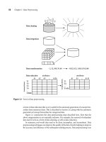
Data matrix (or object-by-variable structure): This represents n objects, such as per-
sons, with p variables (also called measurements or attributes), such as age, height,
weight, gender, and so on. The structure is in the form of a relational table, or n-by-p
matrix (n objects ×p variables):








x
11
··· x
1 f
··· x
1p
··· ··· ··· ··· ···
x
i1
··· x
i f
··· x
ip
··· ··· ··· ··· ···
x
n1
··· x

n f
··· x
np








(7.1)
Dissimilarity matrix (or object-by-object structure): This stores a collection of prox-
imities that are available for all pairs of n objects. It is often represented by an n-by-n
table: