Advanced wireless networks 4g technologies phần 4 ppsx
Bạn đang xem bản rút gọn của tài liệu. Xem và tải ngay bản đầy đủ của tài liệu tại đây (2.03 MB, 88 trang )
JWBK083-08 JWBK083-Glisic February 23, 2006 3:53 Char Count= 0
EFFECTIVE LINK LAYER CAPACITY 243
0
500
1000
1500
2000
2500
3000
3500
20 22 24 26 28 30 32
Rate (cells/ms)
Bucket size (cells)
0.1
0.01
0.001
0.0001
Figure 8.3 Shaping probability curves for nonsmooth mode.
0
500
1000
1500
2000
2500
3000
3500
20 22 24 26 28 30 32
Rate (cells/ms)
B
(cells)
0.1
0.01
0.001
0.0001
Figure 8.4 Shaping probability curves for smooth mode.
8.2 EFFECTIVE LINK LAYER CAPACITY
In the previous section we discussed the problem of effective characterization of the traffic
source in terms of the parameters which are used to negotiate with the network a certain
level of QoS. Similarly, on the network side, to enable the efficient support of quality of
service (QoS) in 4G wireless networks, it is essential to model a wireless channel in terms of
connection-level QoS metrics such as data rate, delay and delay-violation probability. The
traditional wireless channel models, i.e. physical-layer channel models, do not explicitly
characterize a wireless channel in terms of these QoS metrics. In this section, we discuss
a link-layer channel model referred to as effective capacity (EC) [11]. In this approach, a
wireless link is modeled by two EC functions, the probability of nonempty buffer and the
QoS exponent of a connection. Then, a simple and efficient algorithm to estimate these EC
functions is discussed. The advantage of the EC link-layer modeling and estimation is ease
JWBK083-08 JWBK083-Glisic February 23, 2006 3:53 Char Count= 0
244 EFFECTIVE CAPACITY
of translation into QoS guarantees, such as delay bounds and hence, efficiency in admission
control and resource reservation.
Conventional channel models, discussed in Chapter 3, directly characterize the fluctua-
tions in the amplitude of a radio signal. These models will be referred to as physical-layer
channel models, to distinguish them from the link-layer channel model discussed in this
section. Physical-layer channel models provide a quick estimate of the physical-layer per-
formance of wireless communications systems (e.g. symbol error rate vs SNR). However,
physical-layer channel models cannot be easily translated into complex link-layer QoS
guarantees for a connection, such as bounds on delay. The reason is that these complex QoS
requirements need an analysis of the queueing behavior of the connection, which cannot be
extracted from physical-layer models. Thus, it is hard to use physical-layer models in QoS
support mechanisms, such as admission control and resource reservation.
For these reasons, it was proposed to move the channel model up the protocol stack
from the physical layer to the link layer. The resulting model is referred to as EC link model
because it captures a generalized link-level capacity notion of the fading channel. Figure 8.5
illustrates the difference between the conventional physical-layer and link-layer model. For
simplicity, the ‘physical-layer channel’ will be called the ‘physical channel’ and ‘link-layer
channel’ will be referred to as the ‘link’.
8.2.1 Link-layer channel model
4G wireless systems will need to handle increasingly diverse multimedia traffic, which are
expected to be primarily packet-switched. The key difference between circuit switching
and packet switching, from a link-layer design viewpoint, is that packet switching requires
queueing analysisof thelink. Thus,it becomesimportant tocharacterize theeffect ofthe data
traffic pattern, as well as the channel behavior, on the performance of the communication
system.
QoS guarantees have been heavily researched in the wired networks [e.g. ATM and
Internet protocol (IP) networks]. These guarantees rely on the queueing model shown in
Demodulator
Channel
decoder
Network
access
device
Data
sink
Wireless
channel
Modulator
Channel
encoder
Network
access device
Data
source
Receiver
Received SNR
Physical-layer
channel
Transmitter
Link-layer
channel
Instantaneous channel capacity
log(1 + SNR)
Demodulator
Channel
decoder
Network
access
device
Data
sink
Wireless
channel
Modulator
Channel
encoder
Network
access device
Data
source
Receiver
Received SNR
Physical-layer
channel
Transmitter
Link-layer
channel
Instantaneous channel capacity
log(1 + SNR)
Figure 8.5 Packet-based wireless communication system.
JWBK083-08 JWBK083-Glisic February 23, 2006 3:53 Char Count= 0
EFFECTIVE LINK LAYER CAPACITY 245
Data
source
Rate
μ
A(t)
B
Queue
Q(t)
Capacity
S(t)
Channel
Data
source
Rate
μ
A(t)
Queue
Q(t)
Capacity
S(t)
Channel
Figure 8.6 Queueing system model.
Figure 8.6 and studied in Chapter 6. This figure shows that the source traffic and the network
service are matched using a first-in first-out buffer (queue). Thus, the queue prevents loss of
packets that could occur when the source rate is more than the service rate, at the expense
of increasing the delay. Queueing analysis, which is needed to design appropriate admis-
sion control and resource reservation algorithms, requires source traffic characterization
and service characterization. The most widely used approach for traffic characterization is
to require that the amount of data (i.e. bits as a function of time t) produced by a source
conform to an upper bound, called the traffic envelope, (t). The service characteriza-
tion for guaranteed service is a guarantee of a minimum service (i.e. bits communicated
as a function of time) level, specified by a service curve SC (t)[12]. Functions (t)
and (t) are specified in terms of certain traffic and service parameters, respectively. Ex-
amples include the UPC parameters, discussed in the previous section, used in ATM for
traffic characterization, and the traffic specification (T-SPEC) and the service specification
(R-SPEC) fields used with the resource reservation protocol [12] in IP networks.
A traffic envelope (t) characterizes the source behavior in the following manner: over
any window of size t, the amount of actual source traffic A(t) does not exceed (t) (see
Figure 8.7). For example, the UPC parameters, discussed in Section 8.1, specifies (t)by
(t) = min
λ
(s)
p
t,λ
(s)
s
t + σ
(s)
(8.18)
where λ
(s)
p
is the peak data rate, λ
(s)
s
the sustainable rate, and σ
(s)
= B
s
the leaky-bucket size
[12]. As shown in Figure 8.7, the curve (t) consists of two segments: the first segment
has a slope equal to the peak source data rate λ
(s)
p
, while the second has a slope equal to
the sustainable rate λ
(s)
s
, with λ
(s)
s
<λ
(s)
p
. σ
(s)
is the y-axis intercept of the second segment.
(t) has the property that A(t) ≤ (t) for any time t. Just as (t) upper bounds the source
traffic, a network SC (t) lower bounds the actual service S(t) that a source will receive.
(t) has the property that (t) ≤ S(t) for any time t. Both (t) and (t) are negotiated
during the admission control and resource reservation phase. An example of a network SC
is the R-SPEC curve used for guaranteed service in IP networks
(t) = max
λ
(c)
s
(t − σ
(c)
), 0
=
λ
(c)
s
(t − σ
(c)
)
+
(8.19)
where λ
(c)
s
is the constant service rate, and σ
(c)
the delay (due to propagation delay, link
sharing, and so on). This curve is illustrated in Figure 8.7. (t) consists of two segments;
JWBK083-08 JWBK083-Glisic February 23, 2006 3:53 Char Count= 0
246 EFFECTIVE CAPACITY
l
s
(s)
Γ(t)
Q(t)
D(t)
s(c)
s(s)
l
s
(c)
Ψ(t)
S(t)
Time
t
Actual channel service
Number of bits
A(t)
Time
t
Actual channel service
Number of bits
l
p
(S)
Actual source traffic
t
Figure 8.7 Traffic and service characterization. (Reproduced by permission of IEEE [11].)
the horizontal segment indicates that no packet is being serviced due to propagation delay,
etc., for a time interval equal to the delay σ
(c)
, while the second segment has a slope equal to
the service rate λ
(c)
s
. In the figure, the horizontal difference between A(t) and S(t), denoted
D(τ ), is the delay experienced by a packet arriving at time τ , and the vertical difference
between the two curves, denoted by Q(τ ), is the queue length built up at time τ , due to
packets that have not been served yet.
As discussed in Chapter 4, providing QoS guarantees over wireless channels requires
accurate models of their time-varying capacity, and effective utilization of these models
for QoS support. The simplicity of the SCs discussed earlier motivates us to define the
time-varying capacity of a wireless channel as in Equation (8.19). Specifically, we hope to
lower bound the channel service using two parameters: the channel sustainable rate λ
(c)
s
,
and the maximum fade duration σ
(c)
.
Parameters λ
(c)
s
and σ
(c)
are meant to bein a statistical sense. The maximumfade duration
σ
(c)
is a parameter that relates the delay constraint to the channel service. It determines the
probability sup
t
Pr
{
S(t) <(t)
}
. We will see later that σ
(c)
is specified by the source with
σ
(c)
= D
max
, where D is the delay bound required by the source.
However, physical-layer wireless channel modelsdo not explicitly characterize thechan-
nel intermsof suchlink-layer QoSmetricsas datarate, delayanddelay-violation probability.
For this reason, we are forced to look for alternative channel models.
A problemthat surfaces isthat a wirelesschannel has acapacity that variesrandomly with
time. Thus, an attempt to provide a strict lower bound [i.e. the deterministic SC (t), used
in IP networks] will most likely result in extremely conservative guarantees. For example,
in a Rayleigh or Ricean fading channel, the only lower bound that can be deterministically
guaranteed is a capacity of zero. The capacity here is meant to be delay-limited capacity,
which is the maximum rate achievable with a prescribed delay bound (see Hanly and Tse
[13] for details). This conservative guarantee is clearly useless in practice. Therefore, the
concept of deterministic SC (t) is extended to a statistical version, specified as the pair
{
(t),ε
}
. The statistical SC
{
(t),ε
}
specifies that the service provided by the channel,
denoted
˜
S(t), willalways satisfythe property thatsup
t
Pr
˜
S(t) <(t)
≤ ε. In other words,
ε is the probability that the wireless channel will not be able to support the pledged SC
JWBK083-08 JWBK083-Glisic February 23, 2006 3:53 Char Count= 0
EFFECTIVE LINK LAYER CAPACITY 247
(t), referred to as the outage probability. For most practical values of ε,anonzero SC
(t) can be guaranteed.
8.2.2 Effective capacity model of wireless channels
From the previous discussion we can see that for the QoS control we need to calculate an
SC (t) such that, for a given ε>0, the following probability bound on the channel service
˜
S(t) is satisfied:
sup
t
Pr
˜
S(t) <(t)
≤ ε and (t) =
λ
(c)
s
(t − σ
(c)
)
+
(8.20)
The statistical SC specification requires that we relate its parameters {λ
(c)
s
,σ
(c)
,ε} to the
fading wireless channel, which at the first sight seems to be a hard problem. At this point,
the idea that the SC (t)isadual of the traffic envelope (t) is used [11]. A number of
papers exist on the so-called theory of effective bandwidth [14], which models the statistical
behavior of traffic. In particular, the theory shows that the relation sup
t
Pr
{
Q(t) ≥ B
}
≤ ε
is satisfied forlarge B, by choosingtwo parameters(whichare functionsofthe channelrater)
that depend on the actual data traffic, namely, the probability of nonempty buffer, and the
effective bandwidth of the source. Thus, a source model defined by these two functions
fully characterizes the source from a QoS viewpoint. The duality between Equation (8.20)
and sup
t
Pr
{
Q(t) ≥ B
}
≤ ε indicates that it may be possible to adapt the theory of effective
bandwidth to SC characterization. This adaptation will point to a new channel model, which
will be referred to as the effective capacity (EC) link model. Thus, the EC link model can be
thought of as the dual of the effective bandwidth source model, which is commonly used
in networking.
8.2.2.1 Effective bandwidth
The stochastic behavior of a source traffic can be modeled asymptotically by its effective
bandwidth. Consider an arrival process
{
A(t), t ≥ 0
}
, where A(t) represents the amount of
source data (in bits) over the time interval [0, t). Assume that the asymptotic log-moment
generating function of A(t), defined as
(u) = lim
t→∞
1
t
log E
e
uA(t)
(8.21)
exists for all u ≥ 0. Then, the effective bandwidth function of A(t) is defined as [11, 14]
α(u) =
(u)
u
, ∀u ≥ 0. (8.22)
This becomes more evident if we assume the constant traffic A(t) = A so that Equation
(8.21) gives
(u) = lim
t→∞
1
t
log E
e
uA(t)
= lim
t→∞
1
t
log E
e
uA
= lim
t→∞
uA
t
= u lim
t→∞
A
t
= uα(u)
(8.21a)
Consider now a queue of infinite buffer size served by a channel of constant service rate
r, such as an AWGN channel. Owing to the possible mismatch between A(t) and S(t), the
JWBK083-08 JWBK083-Glisic February 23, 2006 3:53 Char Count= 0
248 EFFECTIVE CAPACITY
queue length Q(t) could be nonzero. As already discussed in Section 8.1 [analogous to
Equation (8.5)] or by using the theory of large deviations [14] , it can be shown that the
probability of Q(t) exceeding a threshold B satisfies
sup
t
Pr
{
Q(t) ≥ B
}
∼ e
−θ
B
(r)B
as B →∞ (8.23)
where f (x) ≈ g(x) means that lim
x→∞
f (x)/g(x) = 1. For smaller values of B, the fol-
lowing approximation, analogous to Equation (8.3), is more accurate [15]:
sup
t
Pr
{
Q(t) ≥ B
}
≈ γ (r)e
−θ
B
(r)B
(8.24)
where both γ (r) and θ
B
(r) are functions of channel capacity r. According to the theory,
γ (r) = Pr
{
Q(t) ≥ 0
}
is the probability that the buffer is nonempty for randomly chosen
time t, while the QoS exponent θ
B
is the solution of α(θ
B
) = r. Thus, the pair of functions
{γ (r),θ
B
(r)}model the source. Note that θ
B
(r) is simply the inverse function corresponding
to the effective bandwidth function α(u).
If the quantity of interest is the delay D(t) experienced by a source packet arriving at
time t, then with same reasoning the probability of D(t) exceeding a delay bound D
max
satisfies
sup
t
Pr
{
D(t) ≥ D
max
}
≈ γ (r)e
−θ(r)D
max
(8.25)
where θ(r) = θ
B
(r) ×r [16]. Thus, the key point is that for a source modeled by the pair
{γ (r),θ(r)}, which has a communication delay bound of D
max
, and can tolerate a delay-
bound violation probability of at most ε, the effective bandwidth concept shows that the
constant channel capacity should be at least r, where r is the solution to ε = γ (r)e
−θ(r)D
max
.
In terms of the traffic envelope (t) (Figure 8.7), the slope λ
(s)
s
= r and σ
(s)
= rD
max
.
In Section 8.1 a simple and efficient algorithm to estimate the source model functions
γ (r) and θ(r) was discussed. In the following section, we use the duality between traffic
modeling {γ (r),θ(r)}, and channel modeling to present an EC link model, specified by a
pair of functions {γ
(c)
(μ),θ
(c)
(μ)}. The intention is to use {γ
(c)
(μ),θ
(c)
(μ)}as the channel
duals of the source functions {γ (r),θ(r)}. Just as the constant channel rate r is used in
source traffic modeling, we use the constant source traffic rate μ in modeling the channel.
Furthermore, we adapt the source estimation algorithm from Section 8.1 to estimate the
link model parameters {γ
(c)
(μ),θ
(c)
(μ)}.
8.2.2.2 Effective capacity link model
Let r(t) be the instantaneous channel capacity at time t. Define
˜
S(t) =
t
0
r(τ)dτ, which is
the service provided by the channel. Note that the channel service
˜
S(t) is different from the
actual service S(t) received by the source;
˜
S(t) only depends on the instantaneous channel
capacity and thus is independentof the arrival A(t). Paralleling the development of Equation
(8.21) and (8.22) we assume that
(c)
(−u) = lim
t→∞
1
t
log E
e
−u
˜
S(t)
(8.26)
JWBK083-08 JWBK083-Glisic February 23, 2006 3:53 Char Count= 0
EFFECTIVE LINK LAYER CAPACITY 249
exists for all u ≥ 0. This assumption is valid, for example, for a stationary Markov-fading
process r(t). Then, the EC function of r(t) is defined as
α
(c)
(u) =
−
(c)
(−u)
u
, ∀u ≥ 0 (8.27)
Consider a queue of infinite buffer size supplied by a data source of constant data rate
μ (see Figure 8.6). The theory of effective bandwidth can be easily adapted to this case.
The difference is that, whereas in the previous case the source rate was variable while the
channel capacity was constant, now the source rate is constant while the channel capacity is
variable. Similar to Equation (8.25), it can be shown that the probability of D(t) exceeding
a delay bound D
max
satisfies
sup
t
Pr
{
D(t) ≥ D
max
}
≈ γ
(c)
(μ)e
−θ
(c)
(μ)D
max
(8.28)
where {γ
(c)
(μ),θ
(c)
(μ)} are functions of source rate μ. This approximation is accurate for
large D
max
, but we will see later in the simulation results, that this approximation is also
accurate even for smaller values of D
max
.
For a given source rate μ, γ
(c)
(μ) = Pr
{
Q(t) ≥ 0
}
is again the probability that the buffer
is nonempty at a randomly chosen time t, while the QoS exponent θ
(c)
(μ) is defined as
θ(μ) = μα
−1
(μ), where α
−1
(·) is the inverse function of α
(c)
(u). Thus, the pair of functions
{γ
(c)
(μ),θ
(c)
(μ)} model the link.
So, if a link that is modeled by the pair {γ
(c)
(μ),θ
(c)
(μ)}is used, a source that requires a
communication delay bound of D
max
, and can tolerate a delay-bound violation probability
of at most ε, needs to limit its data rate to a maximum of μ, where μ is the solution to
ε = γ
(c)
(μ)e
−θ
(c)
(μ)D
max
. In termsof the SC (t) shownin Figure 8.7, thechannel sustainable
rate λ
(c)
s
= μ and σ
(c)
= D
max
.
If the channel-fading process r(t) is stationary and ergodic, then a simple algorithm
to estimate the functions {γ
(c)
(μ),θ
(c)
(μ)} is similar to the one described in Section 8.1.
Paralleling Equation (8.7) we have
γ
(c)
(μ)
θ
(c)
(μ)
= E
[
D(t)
]
= τ
s
(μ) +
E
[
Q(t)
]
μ
(8.29)
γ
(c)
(μ) = Pr
{
D(t) > 0
}
(8.30)
where τ
s
(μ) is the average remaining service time of a packet being served. Note that τ
s
(μ)
is zero for a fluid model (assuming infinitesimal packet size). Now, the delay D(t) is the sum
of the delay incurred due to the packet already in service, and the delay in waiting for the
queue Q(t) to clear which results in Equation (8.29), using Little’s theorem. Substituting
D
max
= 0 in Equation (2.28) results in Equation (3.30). As in Section 8.1, solving Equation
(8.29) for θ
(c)
(μ) gives similarly to Equation (8.8a)
θ
(c)
(μ) =
γ
(c)
(μ) ×μ
μ ×τ
s
(μ) + E
[
Q(t)
]
(8.31)
According to Equation (8.30) and (8.31) , as in Section 8.1, the functions γ and θ can be
estimated by estimating Pr
{
D(t) > 0
}
,τ
s
(μ), and E
[
Q(t)
]
. The latter can be estimated
by taking a number of samples, say N, over an interval of length T , and recording the
following quantities at the nth sampling epoch: S
n
the indicator of whether a packets is in
service (S
n
∈
{
0, 1
}
), Q
n
the number of bits in the queue (excluding the packet in service),
JWBK083-08 JWBK083-Glisic February 23, 2006 3:53 Char Count= 0
250 EFFECTIVE CAPACITY
and T
n
the remaining service time of the packet in service (if there is one in service). Based
on the same measurements, as in Section 8.1,
ˆγ =
N
n=1
S
n
/N
ˆ
q =
N
n=1
Q
n
/N
ˆτ
s
=
N
n=1
T
n
/N
are computed and then, from Equation (8.31), we have
ˆ
θ =
ˆγ ×μ
μ × ˆτ
s
+
ˆ
q
(8.32)
These parameters are used to predict the QoS by approximating Equation (8.28) with
sup
t
Pr
{
D(t) ≥ D
max
}
≈ ˆγ e
−
ˆ
θ D
max
(8.33)
If the ultimate objective of EC link modeling is to compute an appropriate SC (t), then,
given the delay-bound D
max
and the target delay-bound violation probability ε of a connec-
tion, we can find (t) ={σ
(c)
,λ
(c)
s
} by setting σ
(c)
= D
max
, solving Equation (8.33) for μ
and setting λ
(c)
s
= μ.
8.2.3 Physical layer vs link-layer channel model
In Jack’s model of a Rayleigh flat-fading channel, the Doppler spectrum S( f )isgivenas
S( f ) =
1.5
π f
m
1 −
(
F/ f
m
)
2
(8.34)
where f
m
is the maximum Doppler frequency, f
c
is the carrier frequency, and F = f − f
c
.
Below we show how to calculate the EC for this channel [11].
Denote a sequence of N measurements of the channel gain, spaced at a time interval
δ apart, by x =
[
x
0
, x
1
, ···, x
N−1
]
, where
{
x
n
, n ∈
[
0, N − 1
]
}
are the complex-valued
Gaussian distributed channel gains(
|
x
n
|
are, therefore, Rayleighdistributed). For simplicity,
the constant noise variance will be included in the definition of x
n
. The measurement x
n
is a realization of a random variable sequence denoted by X
n
, which can be written as the
vector X =
[
X
0
, X
1
, ···, X
N−1
]
. The pdf of a random vector X for the Rayleigh-fading
channel is
f
X
(X) =
1
π
N
det(R)
e
−xR
−1
x
H
(8.35)
where R is the covariance matrix of the random vector X, det(R) the determinant of matrix
R, and x
H
the conjugate transpose (Hermitan) of x. To calculate the EC, we start with
E[e
−u
˜
S(t)
] = E
exp
−u
t
0
r(τ)dτ
(a)
≈
exp
−u
N−1
n=0
δ × r(τ
n
)
f
x
(x)dx
JWBK083-08 JWBK083-Glisic February 23, 2006 3:53 Char Count= 0
EFFECTIVE LINK LAYER CAPACITY 251
(b)
≈
exp
−u
N−1
n=0
δ log(1 +|x
n
|
2
)
f
x
(x)dx (8.36)
(c)
≈
exp
−u
N−1
n=0
δ log(1 +|x
n
|
2
)
.
1
π
N
det(R)
e
−xR
−1
x
H
dx
where (a) approximates the integral by a sum, (b) is the Shannon result for channel capacity
(i.e. γ (τ
n
) = log(1 +
|
x
n
|
2
), and (c) is from Equation (8.35). This gives the EC, Equation
(8.27), as
α
(c)
(u) =
−1
u
lim
t→∞
log
exp
−u
N−1
n=0
δ log(1 +|x
n
|
2
)
.
1
π
N
det(R)
e
−xR
−1
x
H
dx
(8.37)
Using the approximation (a) log(1 +
|
x
n
|
2
) ≈
|
x
n
|
2
for low SNR [11], Equation (8.37) can
be further simplified as
E[e
−u
˜
S(t)
]
(a)
≈
exp
−uδ
N−1
n=0
|x
n
|
2
.
1
π
N
det(R)
e
−xR
−1
x
H
dx
(b)
=
e
−uδ||x||
2
1
π
N
det(R)
e
−xR
−1
x
H
dx
(b)
=
1
π
N
det(R)
e
−x(R
−1
+uδI)x
H
dx (8.38)
=
1
π
N
det(R)
× π
N
det
(R
−1
+ uδI)
−1
=
1
det(uδR + I)
where approximation (b) is due to the definition of the norm of the vector x, and (c) the
relation
x
2
= xx
H
(I is identity matrix). Reference [11] considers three cases of interest
for Equation (8.38).
8.2.3.1 High mobility scenario
In the extreme high mobility (HM) case there is no correlation between the channel samples
and we have R = rI, where r = E
|
x
n
|
2
is the average channel capacity. From Equation
(8.38), we have
E[e
−u
˜
S(t)
] ≈
1
det(uδR + I)
=
1
(urδ +1)
N
=
1
(urt/N + 1)
N
(8.39)
where δ t/N. As the number of samples N →∞,wehave
lim
N→∞
E[e
−u
˜
S(t)
] ≈ lim
N→∞
(urt/N + 1)
−N
= e
−urt
(8.40)
Thus, in the limiting case, the Rayleigh-fading channel reduces to an AWGN channel. Note
that this result would not apply at high SNRs because of the concavity of the log(·) function.
JWBK083-08 JWBK083-Glisic February 23, 2006 3:53 Char Count= 0
252 EFFECTIVE CAPACITY
8.2.3.2 Stationary scenario
In this case all the samples are fully correlated, R = [R
ij
] = [r]. In other words all elements
of R are the same and Equation (8.38) now gives
E[e
−u
˜
S(t)
] ≈
1
det(uδR + I)
=
1
urδN + 1
=
1
ur ×
t
N
× N + 1
=
1
1 +urt
(8.41)
8.2.3.3 General case
Denote the eigenvalues of matrix R by {λ
n
, n ∈
[
0, N − 1
]
}. Since R is symmetric, we
have R = UDU
H
, where U is a unitary matrix, U
H
is its Hermitian, and the diagonal matrix
D = diag
(
λ
0
,λ
1
, ···,λ
N−1
)
. From Equation (8.38), we have
E[e
−u
˜
S(t)
] ≈
1
det(uδR + I)
=
1
det(uδUDU
H
+ UU
H
)
=
1
det[U diag (uδλ
0
+ 1, uδλ
1
+ 1, ,uδλ
N−1
+ 1)U
H
]
=
1
n
(uδλ
n
+ 1)
= exp
−
n
log(uδλ
n
+ 1)
(8.42)
We now use the calculated E[e
−u
˜
S(t)
]toget
(c)
(−u) = lim
t→∞
1
t
log E[e
−u
˜
S(t)
]
(a)
≈
lim
t→∞
1
t
log exp
−
n
log(uδλ
n
+ 1)
(b)
=
lim
f →0
− f
n
log
u
λ
n
B
w
+ 1
(c)
=
−
log(uS( f ) + 1) d f (8.43)
where (a) follows from Equation (8.42), (b) follows from the fact that the frequency interval
f = 1/t and the bandwidth B
w
= 1/δ, and (c) from the fact thatthe power spectral density
S( f ) = λ
n
/B
w
and that the limit of a sum becomes an integral. This gives the EC, Equation
(8.27), as
α
(c)
(u) =
log(uS( f ) + 1)d f
u
(8.44)
Thus, the Dopplerspectrum allows us to calculate α
(c)
(u). The EC function,Equation (8.44),
can be used to guarantee QoS using Equation (8.28).
One should keep inmindthat theECfunction, Equation(8.44),is validonly foraRayleigh
flat-fading channel, at low SNR. At high SNR, the EC for a Rayleigh-fading channel is
specified by the complicated integral in Equation (8.37). To the best of our knowledge, a
closed-form solution toEquation (8.37) does not exist. Itis clear that anumerical calculation
of EC is also very difficult, because the integral has a high dimension. Thus, it is difficult to
extract QoS metrics from a physical-layer channel model, even for a Rayleigh flat-fading
channel. The extraction may not even be possible for more general fading channels. In
contrast, the EC link model that was described in this section can be easily translated into
QoS metrics for a connection, and we have shown a simple estimation algorithm to estimate
the EC model functions.
JWBK083-08 JWBK083-Glisic February 23, 2006 3:53 Char Count= 0
EFFECTIVE LINK LAYER CAPACITY 253
Data
source
Rate =
μ
Q
n
r
n
Transmitter
Transmitted
data
Gain
Noise
Fading
channel
Receiver
Received
signal
Data
source
Rate =
μ
Q
n
r
n
Transmitter
Transmitted
data
Gain
Noise
Fading
channel
Receiver
Received
signal
Figure 8.8 Queueing model used for simulations.
8.2.4 Performance examples
The discrete-time system depicted in Figure 8.8 is simulated. The data source generates
packets at a constant rate μ which are first sent to the (infinite) buffer at the transmitter,
whose queue length is Q
n
, where n refers to the nth sample interval. The head-of-line packet
in the queue is transmitted over the fading channel at data rate r
n
. The fading channel has
a random channel gain x
n
(the noise variance is absorbed into x
n
). We use a fluid model
that is the size of a packet is infinitesimal. A perfect knowledge of the channel gain x
n
(the
SNR, really) at the transmitter side is assumed. Therefore, as described in Chapter 4, it
can use rate-adaptive transmissions and strong channel coding to transmit packets without
errors. Thus, the transmission rate r
n
is equal to the instantaneous (time-varying) capacity
of the fading channel, defined by the Shannon law, r
n
= B
c
log
2
(1 +|x
n
|
2
) where B
c
is the
channel bandwidth.
The average SNR is fixed in each simulation run. We define r
g
as the capacity of an
equivalentAWGNchannel,which has thesame averageSNR, i.e.r
g
= B
c
log
2
(1 +SNR
avg
)
where SNR
avg
is the average SNR, i.e. E
|
x
n
|
2
. Then, r
n
/r
g
relation
r
n
=
r
awgn
log
2
(1 +|x
n
|
2
)
log
2
(1 +SNR
avg
)
(8.45)
Simulation parameters as in Wu and Negi [11] were used. Channel samples x
n
are gener-
ated by the following AR(1) (autoregressive) model: x
n
= kx
n−1
+ v
n
where the modeling
error v
n
is zero-mean complex Gaussian with unit variance per dimension and is statisti-
cally independent of x
n−1
. The coefficient k can be determined by the following procedure:
(1) compute thecoherence time T
c
by T
c
≈ 9/16π f
m
, where thecoherence time is definedas
the time over which the time autocorrelation function of the fading process is above 0.5; (2)
JWBK083-08 JWBK083-Glisic February 23, 2006 3:53 Char Count= 0
254 EFFECTIVE CAPACITY
0
0.2
0.4
0.6
0.8
1
30 40 50 60 70 80
Source rate (kb/s)
Parameter
0
1
30 40 50 60 70 80
Source rate (kb/s)
Parameter
SNR
avg
= 0 dB, f
m
= 5 Hz
SNR
avg
= 0 dB, f
m
= 30 Hz
SNR
avg
= 15 dB, f
m
= 5 Hz
SNR
avg
= 15 dB, f
m
= 30 Hz
Figure 8.9 Estimated function ˆγ (μ) vs source rate μ.
compute the coefficient k by k = 0.5
T
s
/T
c
where T
s
is the sampling interval. The other pa-
rameters are: f
m
= 5–30 Hz, r
g
= 100 kb/s, average SNR = 0/15 dB, T
s
= 1 ms, bit rate
μ = 30–85 kb/s.
Figures 8.9 and 8.10 show the estimated EC functions ˆγ (μ) and
ˆ
θ(μ). As the source
rate μ increases from 30 to 85 kb/s, ˆγ (μ) increases, indicating a higher buffer occupancy,
while
ˆ
θ(μ) decreases, indicating a slower decay of the delay-violation probability. Thus,
the delay-violation probability is expected to increase with increasing source rate μ. From
Figure 8.10, we also observe that SNR has a substantial impact on ˆγ (μ). This is because
higher SNR results in larger channel capacity, which leads to smaller probability that a
packet will be buffered, i.e. smaller ˆγ (μ). In contrast, Figure 8.9 shows that f
m
has little
effect on ˆγ (μ).
SNR
avg
= 0 dB, f
m
= 5 Hz
SNR
avg
= 0 dB, f
m
= 30 Hz
SNR
avg
= 15 dB, f
m
= 5 Hz
SNR
avg
= 15 dB, f
m
= 30 Hz
10
-4
10
-3
10
-2
10
-1
10
0
30
40
50
60
70
80
Source rate (kb/s)
Parameter
Figure 8.10 Estimated function
ˆ
θ(μ) vs source rate μ.
JWBK083-08 JWBK083-Glisic February 23, 2006 3:53 Char Count= 0
REFERENCES 255
50
10
-3
10
-2
10
-1
10
0
10
-3
10
-2
10
-1
10
0
100
Delay bound D
max
(ms)
200 250
300150
50
100
Delay bound D
max
(ms)
200 250
300150
f
m
=5
f
m
=10
f
m
=15
f
m
=30
Probability Pr{D(t)>D
max
}
Probability Pr{D(t)>D
max
}
Figure 8.11 Actual delay-violation probability vs D
max
for various Doppler rates. (a)
Rayleigh fading and (b) Ricean fading K = 3.
Figure 8.11 shows the actual delay-violation probability sup
t
Pr{D(t) > D
max
} vs the
delay bound D
max
, for various Doppler rates. It can be seen that the actual delay-violation
probability decreases exponentially with the delay bound D
max
, for all the cases. This justi-
fies the use of an exponential bound, Equation (8.33), in predicting QoS, thereby justifying
the link model {ˆγ,
ˆ
θ}. The figure shows that delay-violation probability reduces with the
Doppler rate. This is reasonable since the increase of the Doppler rate leads to the increase
of time diversity, resulting in a larger decay rate
ˆ
θ(μ) of the delay-violation probability.
More details on the topic can be found in References [11–17].
REFERENCES
[1] ATM Forum Technical Committee, Traffic Management Specification, Version 4.0.
ATM Forum, 1996.
[2] A.I. Elwalid and D. Mitra, Analysis and design of rate-based congestion control of
high speed networks – I: stochastic fluid models, access regulation, Queueing Syst.,
vol. 9, 1991, pp. 29–63.
[3] J.S. Turner,New directions incommunications (or which way to theinformation age?),
IEEE Commun. Mag., 1986, pp. 8–15.
[4] R.L. Cruz, A calculus for network delay, part I: network elements in isolation, IEEE
Trans. Inform. Theory, vol. 37, 1991, pp. 114–131.
[5] B.L. Mark, and G. Ramamurthy, Real-time estimation and dynamic renegotiation of
UPC parameters for arbitrary traffic sources in ATM networks, IEEE/ACM Trans.
Networking, vol. 6, no. 6, 1998, pp. 811–828.
[6] C. Chang, Stability, queue length and delay of deterministic and stochastic queueing
networks, IEEE Trans. Automat. Contr., vol. 39, 1994, pp. 913–931.
[7] G.L. Choudhury, D.M. Lucantoni and W. Whitt, Squeezing the most out of ATM,
IEEE Trans. Commun., vol. 44, 1996, pp. 203–217.
JWBK083-08 JWBK083-Glisic February 23, 2006 3:53 Char Count= 0
256 EFFECTIVE CAPACITY
[8] P.W. Glynn and W. Whitt, Logarithmic asymptotics for steadystate tail probabilities
in a single-server queue, in Studies in Applied Probability, Papers in Honor of Lajos
Takacs, J. Galambos and J. Gani, eds, Applied Probability Trust, 1994, pp. 131–
156.
[9] H. Kobayashi and Q. Ren, A diffusion approximation analysis of an ATM statistical
multiplexer with multiple types of traffic, part I: equilibrium state solutions, in Proc.
1993 IEEE Int. Conf. Communications, Geneva, May 1993, vol. 2, pp. 1047–1053.
[10] B.L. Mark and G. Ramamurthy, Joint source-channel control for realtime VBR
over ATM via dynamic UPC renegotiation, in Proc. IEEE Globecom’96, London,
November, 1996, pp. 1726–1731.
[11] D. Wu, and R. Negi, Effective capacity: a wireless link model for support of quality
of service, IEEE Trans. Wireless Commun., vol. 2, no. 4, 2003, pp. 630–643.
[12] R. Guerin and V. Peris, Quality-of-service in packet networks: Basic mechanisms and
directions, Comput. Networks, ISDN, vol. 31, no. 3, 1999, pp. 169–179.
[13] S. Hanly and D. Tse, Multiaccess fading channels: Part II: Delay-limited capacities,
IEEE Trans. Inform. Theory, vol. 44, 1998, pp. 2816–2831.
[14] C S. Chang and J.A. Thomas, Effective bandwidth in high-speed digital networks,
IEEE J. Select. Areas Commun., vol. 13, 1995, pp. 1091–1100.
[15] G.L. Choudhury, D.M. Lucantoni and W. Whitt, Squeezing the most out of ATM,
IEEE Trans. Commun., vol. 44, 1996, pp. 203–217.
[16] Z L. Zhang, End-to-end support for statistical quality-of-service guarantees in multi-
media networks, Ph.D. dissertation, Department of Computer Science, University of
Massachusetts, 1997.
[17] B. Jabbari, Teletraffic aspectsof evolving and next-generation wirelesscommunication
networks, IEEE Pers. Commun., vol. 3, 1996, pp. 4–9.
[18] S. Chong and S. Li, (σ ; ρ)-characterization based connection control for guaranteed
services in high speed networks, in Proc. IEEE INFOCOM’95, Boston, MA, April
1995, pp. 835–844.
[19] O. Yaron andM. Sidi, Performanceand stability ofcommunication networks viarobust
exponential bounds, IEEE/ACM Trans. Networking, vol. 1, 1993, pp. 372–385.
[20] T. Tedijanto and L. Gun, Effectiveness of dynamic bandwidth management in ATM
networks, in Proc. INFOCOM’93, San Francisco, CA, March 1993, pp. 358–367.
[21] M. Grossglauser, S. Keshav, and D. Tse, RCBR: a simple and efficient service for
multiple time-scale traffic, in Proc. ACM SigCom’95, Boston, MA, August 1995,
pp. 219–230.
[22] D. Reininger, G. Ramamurthy and D. Raychaudhuri, VBR MPEG video coding with
dynamic bandwidth renegotiation, in Proc. ICC’95, Seattle, WA, June 1995,pp. 1773–
1777.
[23] J. Abate, G.L. Choudhury, and W. Whitt, Asymptoticsfor steady-state tail probabilities
in structured Markov queueing models, Stochastic Models, vol. 10, 1994, pp. 99–143.
[24] D.P. Heyman and T.V. Lakshman, What are the implications of long-range depen-
dence for VBR-video traffic engineering? IEEE/ACM Trans. Networking, vol. 4, 1996,
pp. 301–317.
[25] W. Whitt, Tail probabilities with statistical multiplexing and effective bandwidths in
multi-class queues, Telecommun. Syst., vol. 2, 1993, pp. 71–107.
[26] D.E. Knuth, The Art of Computer Programming, Volume 2: Seminumerical Algo-
rithms, 2nd edn. Addison-Wesley: Reading, MA, 1981.
JWBK083-08 JWBK083-Glisic February 23, 2006 3:53 Char Count= 0
REFERENCES 257
[27] A.I. Elwalid and D. Mitra, Effective bandwidth of general Markovian traffic sources
and admission control of high speed networks, IEEE/ACM Trans. Networking, vol. 1,
1993, pp. 323–329.
[28] A.K. Parekh and R.G. Gallager, A generalized processor sharing approach to flow
control in integrated services networks: The singlenode case, IEEE/ACM Trans. Net-
working, vol. 1, 1993, pp. 344–357.
[29] B.L. Mark and G. Ramamurthy, UPC-based traffic descriptors for ATM: How to de-
termine, interpret and use them, Telecommun. Syst., vol. 5, 1996, pp. 109–122.
JWBK083-08 JWBK083-Glisic February 23, 2006 3:53 Char Count= 0
258
JWBK083-09 JWBK083-Glisic February 23, 2006 3:55 Char Count= 0
9
Adaptive TCP Layer
9.1 INTRODUCTION
In this section we first discuss TCP performance independent of the type of network by
considering the different possible characteristics of the connection path. We present the
problems and the different possible solutions. This study permits us to understand the
limitations of the actual solutions and the required modifications to let TCP cope with a
heterogeneous Internet on an end-to-end basis. Then, in the rest of the chapter we focus on
the specifics of TCP operation in wireless networks.
The TCP provides a reliable connection-oriented in-order service to many of today’s
Internet applications. Given the simple best-effort service provided by IP, TCP must cope
with the different transmission media crossed by Internet traffic. This mission of TCP is
becoming difficult with the increasing heterogeneity of the Internet. Highspeed links (optic
fibers), long and variable delay paths (satellite links), lossy links (wireless networks) and
asymmetric paths (hybridsatellite networks) arebecoming widely embedded inthe Internet.
Many works have studied by experimentation [1], analytical modeling [2] and simulation
[3, 4, 12, 17, 18] the performance of TCP in this new environment.
Most of these works have focused on a particular environment (satellite networks, mo-
bile networks, etc.). They have revealed some problems in the operation of TCP. Long
propagation delay and losses on a satellite link, handover and fading in a wireless net-
work, bandwidth asymmetry in some media, and other phenomena have been shown to
seriously affect the throughput of a TCP connection. A large number of solutions have been
proposed. Some solutions suggest modifications to TCP to help it to cope with these new
paths. Other solutions keep the protocol unchanged and hide the problem from TCP. In this
section we consider the different characteristics of a path crossed by TCP traffic, focusing
on bandwidth-delay product (BDP), RTT, noncongestion losses and bandwidth asymmetry.
TCP is a reliable window-based ACK-clocked flow control protocol. It uses an additive-
increase multiplicative-decrease strategy for changing its window as a function of network
Advanced Wireless Networks: 4G Technologies Savo G. Glisic
C
2006 John Wiley & Sons, Ltd.
259
JWBK083-09 JWBK083-Glisic February 23, 2006 3:55 Char Count= 0
260 ADAPTIVE TCP LAYER
conditions. Starting from one packet, or a larger value as we will see later, the window is
increased by one packet for every nonduplicate ACK until the source estimate of network
propagation time (npt) is reached. By the propagation time of the network, sometimes called
the pipe size, we mean the maximum number of packets that can be fit on the path, which is
also referred to as network capacity. This is the slow start (SS) phase, and the npt estimate
is called the SS threshold (sst). SS aims to alleviate the burstiness of TCP while quickly
filling the pipe. Once sst is reached, the source switches to a slower increase in the window
by one packet for every window’s worth of ACKs. This phase, called congestion avoidance
(CA), aims to slowly probe the network for any extra bandwidth. The window increase
is interrupted when a loss is detected. Two mechanisms are available for the detection of
losses: the expiration of a retransmission timer (timeout) or the receipt of three duplicate
ACKs (fast retransmit, FRXT). The source supposes that the network is in congestion and
sets its estimate of the sst to half the current window.
Tahoe, the first version of TCP to implement congestion control, at this point sets the
window to one packet and uses SS to reach the new sst. Slow starting after every loss
detection deteriorates the performancegiven the low bandwidth utilizationduring SS. When
the loss is detected via timeout, SS is unavoidable since the ACK clock has stopped and SS
is required to smoothly fill the pipe. However, in the FRXT case, ACKs still arrive at the
source and losses can be recovered without SS. This is the objective of the new versions
of TCP (Reno, New Reno, SACK, etc.), discussed in this chapter, that call a fast recovery
(FRCV) algorithm to retransmit the losses while maintaining enough packets in the network
to preserve the ACK clock. Once losses are recovered, this algorithm ends and normal CA
is called. If FRCV fails, the ACK stream stops, a timeout occurs, and the source resorts to
SS as with Tahoe.
9.1.1 A large bandwidth-delay product
The increaseinlink speed,like inoptic fibers,hasled topaths oflargeBDP. TheTCP window
must be able to reach large values in order to efficiently use the available bandwidth. Large
windows, up to 2
30
bytes, are now possible. However, at large windows, congestion may
lead to the loss of many packets from the same connection. Efficient FRCV is then required
to correct many losses from the same window. Also, at large BDP, network buffers have
an important impact on performance. These buffers must be well dimensioned and scale
with the BDP. Fast recovery uses the information carried by ACKs to estimate the number
of packets in flight while recovering from losses. New packets are sent if this number falls
below the network capacity estimate. The objective is to preserve the ACK clock in order to
avoid the timeout. The difference between the different versions of TCP is in the estimation
of the number of packets in flight during FRCV. All these versions will be discussed later in
more detail. Reno considers every duplicate ACK a signal that a packet has left the network.
The problem of Reno is that it leaves FRCV when an ACK for the first loss in a window
is received. This prohibits the source from detecting the other losses with FRXT. A long
timeout is required to detect the other losses. New Reno overcomes this problem. The idea
is to stay in FRCV until all the losses in the same window are recovered. Partial ACKs are
used to detect multiple losses in the same window. This avoids timeout but cannot result
in a recovery faster than one loss per RTT. The source needs to wait for the ACK of the
retransmission to discover the next loss. Another problem of Reno and New Reno is that
JWBK083-09 JWBK083-Glisic February 23, 2006 3:55 Char Count= 0
INTRODUCTION 261
they rely on ACKs to estimate the number of packets in flight. ACKs can be lost on the
return path, which results in an underestimation of the number of packets that have left
the network, and thus an underutilization of the bandwidth during FRCV and, in the case
of Reno, a possible failure of FRCV. More information is needed at the source to recover
faster than one loss per RTT and to estimate more precisely the number of packets in the
pipe. This information is provided by selective ACK (SACK), a TCP option containing the
three blocks of contiguous data most recently received at the destination. Many algorithms
have been proposed to use this information during FRCV. TCP-SACK may use ACKs to
estimate the number of packets in the pipe and SACKs to retransmit more than one loss
per RTT. This leads to an important improvement in performance when bursts of losses
appear in the same window, but the recovery is always sensitive to the loss of ACKs. As
a solution, forward ACK (FACK) may be used, which relies on SACK in estimating the
number of packets in the pipe. The number and identity of packets to transmit during FRCV
is decoupled from the ACK clock, in contrast to TCP-SACK, where the identity is only
decoupled.
9.1.2 Buffer size
SS results in bursts of packets sent at a rate exceeding the bottleneck bandwidth. When
the receiver acknowledges every data packet, the rate of these bursts is equal to twice the
bottleneck bandwidth. If network buffers are not well dimensioned, they will overflow early
during SS before reaching the network capacity. This will result in an underestimation of
the available bandwidth and a deterioration in TCP performance. Early losses during SS
were first analyzed in Lakshman and Madhow [2]. The network is modeled with a single
bottleneck node of bandwidth μ, buffer B, and two-way propagation delay T , as shown in
Figure 9.1.
A long TCP-Tahoe connection is considered where the aim of SS is to reach quickly
without losses sst,which is equal to half the pipe size [(B + μT )/2]. In the case of a
receiver thatacknowledges every datapacket, they foundthat a buffer B > BDP/3 = μT/3
is required. Their analysis can be extended to an SS phase with a different threshold, mainly
to that at the beginning of the connection, where sst is set to a default value. As an example,
the threshold can be set at the beginning of the connection to the BDP in order to switch to
CA before the occurrence of losses. This will not work if the buffer is smaller than half
the BDP (half μT/2). In Barakat and Altman [5] the problem of early buffer overflow
during SS for multiple routers was studied. It was shown that, due to the high rate at which
source
μ
Desti-
nation
B
T
Source
μ
Desti-
nation
B
T
Figure 9.1 One-hop TCP operation.
JWBK083-09 JWBK083-Glisic February 23, 2006 3:55 Char Count= 0
262 ADAPTIVE TCP LAYER
packets are sent during SS, queues can build up in routers preceding the bottleneck as well.
Buffers in these routers must also be well dimensioned, otherwise they overflow during
SS and limit the performance even though they are faster than the bottleneck. With small
buffers, losses during SS are not a signal of network congestion, but rather of transient
congestion due to the bursty nature of SS traffic. Now in CA, packets are transmitted at
approximately the bottleneck bandwidth. A loss occurs when the window reaches the pipe
size. Thesource divides itswindow by two andstarts a new cycle. To always geta throughput
approximately equal to the bottleneck bandwidth, the window after reduction must be larger
than the BDP. This requires a buffer B larger than the BDP. Note that we are talking about
drop tail buffers, which start to drop incoming packets when the buffer is full. Active buffers
such as random early detection (RED) [3] start to drop packets when the average queue
length exceeds some threshold. When an RED buffer is crossed by a single connection, the
threshold should be larger than the BDP to get good utilization. This contrasts one of the
aims of RED: limiting the size of queues in network nodes in order to reduce end-to-end
delay. For multiple connections, a lower threshold is sufficient given that a small number of
connections reduce their windows upon congestion, in contrast to drop tail buffers, where
often all the connections reduce their windows simultaneously .
9.1.3 Round-trip time
Long RTTs are becoming an issue with the introduction of satellite links into the Internet. A
long RTT reduces the rate at which the window increases, which is a function of the number
of ACKs received and does not account for the RTT. This poses many problems to the
TCP. First, it increases the duration of SS, which is a transitory phase designed to quickly
but smoothly fill the pipe. Given the low bandwidth utilization during SS, this deteriorates
the performance of TCP transfers, particularly short ones (e.g. Web transfers). Second, it
causes unfairness in the allocation of the bottleneck bandwidth. Many works have shown
the bias of TCP against connections with long RTTs [2]. Small RTT connections increase
their rates more quickly and grab most of the available bandwidth. The average throughput
of a connection has been shown to vary as the inverse of T
α
, where α is a factor between 1
and 2 [2].
Many solutions have been proposed to reduce the time taken by SS on long delay
paths. These solutions can be divided into three categories: (1) change the window increase
algorithm of TCP; (2) solve the problem at the application level; or (3) solve it inside the
network. On the TCP level the first proposition was to use a larger window than one packet
at the beginning of SS. An initial window of maximum four packets has been proposed.
Another proposition, called byte counting, was to account for the number of bytes covered
by an ACK while increasing the window rather than the number of ACKs. To avoid long
bursts in the case of large gaps in the ACK stream, a limit on the maximum window increase
has been proposed (limited byte counting). These solutions try to solve the problem while
preserving the ACK clock. They result in an increase in TCP burstiness and an overload on
network buffers. Another type of solution tries to solve the problem by introducing some
kind of packet spacing (e.g. rate-based spacing). The source transmits directly at a large
window without overloading the network. Once the large window is reached, theACK clock
takes over. This lets the source avoid a considerable part of SS. The problem can be solved
at the application level without changing the TCP. A possible solution (e.g. XFTP), consists
of establishing many parallel TCP connections for the same transfer. This accelerates the
JWBK083-09 JWBK083-Glisic February 23, 2006 3:55 Char Count= 0
INTRODUCTION 263
destination
B
A
source
TCP Conection 1
TCP Conection 2
Optimized transport
protocol, no slow start
Suppression of
destination ACKs
Generation of ACKs
Long delay link
Destination
B
A
Source
n
io
Figure 9.2 Spoofing: elimination of the long delay link from the feedback loop.
growth of the resultant window, but increases the aggressiveness of the transfer and hence
the losses in the network. An adaptive mechanism has been proposed for XFTP to change
the number of connections as a function of network congestion. Another solution has been
proposed to accelerate the transfer of web pages. Instead of using an independent TCP
connection to fetch every object in a page, the client establishes a persistent connection and
asks the server to send all the objects on it (hypertext transfer protocol, HTTP). Only the
first object suffers from the long SS phase; the remaining objects are transferred at a high
rate. The low throughput during SS is compensated for by the long time remaining in CA.
The problem can be also solved inside the network rather than at hosts, which is worth-
while when a long delay link is located on the path. In order to decrease the RTT, the long
delay link is eliminated from the feedback loop by acknowledging packets at the input of
this link (A in Figure. 9.2). Packets are then transmitted on the long delay link using an
optimized transport protocol (e.g. STP, described in Henderson and Katz [1]).
This transport protocol is tuned to quickly increase its transmission rate without the need
for a long SS.Once arriving at the output (B), another TCP connectionis used to transmit the
packets to the destination. In a satellite environment, the long delay link may lead directly
to the destination, so another TCP connection is not required. Because packets have already
been acknowledged, any loss between the input of the link (A) and the destination must be
locally retransmitted on behalf the source. Also, ACKs from the receiver must be discarded
silently (at B) so as not to confuse the source. This approach is called TCP spoofing. The
main gain in performance comes from not using SS on the long delay link. The window
increases quickly, which improves performance, but spoofing still has many drawbacks.
First, it breaks the end-to-end semantics of TCP; a packet is acknowledged before reaching
its destination. Also, it does not work when encryption is accomplished at the IP layer,
and it introduces a heavy overload on network routers. Further, the transfer is vulnerable to
path changes, and symmetric paths are required to be able to discard the ACKs before they
reach the source. Spoofing can be seen as a particular solution to some long delay links.
It is interesting when the long delay link is the last hop to the destination. This solution is
often used in networks providing high-speed access to the Internet via geostationary earth
orbit (GEO) satellite links.
JWBK083-09 JWBK083-Glisic February 23, 2006 3:55 Char Count= 0
264 ADAPTIVE TCP LAYER
9.1.4 Unfairness problem at the TCP layer
One way to solve the problem is action at the TCP level by accelerating the window
growth for long RTT connections. An example of a TCP-level solution is, the constant rate
algorithm. The window is increased in CA by a factor inversely proportional to
(
RTT
)
2
.
The result is a constant increase rate of the throughput regardless of RTT, thus better
fairness. The first problem in this proposition is the choice of the increase rate. Also,
accelerating window growth while preserving the ACK clock results in large bursts for long
RTT connections.
Inside the network, fairness is improved by isolating the different connections from
each other. Given that congestion control in TCP is based on losses, isolation means that
a congested node must manage its buffer to distribute drops on the different connections
in such a way that they get the same throughput. Many buffer management policies have
been proposed. Some of these policies, such as RED (random early detection) [3], drop
incoming packets with a certain probability when the queue length or its average exceeds
a certain threshold. This distributes losses on the different connections proportionally to
their throughput without requiring any per-connection state. However, dropping packets in
proportion to the throughput does not always lead to fairness, especially if the bottleneck
is crossed by unresponsive traffic. With a first-in first-out (FIFO) scheduler, the connection
share of the bandwidth is proportional to its share of the buffer. Better fairness requires
control of the buffer occupancy of each connection. Another set of policies, known as Flow
RED, try to improve fairness by sharing the buffer space fairly between active connections.
This ensures that each connection has at least a certain number of places in the queue, which
isolates connections sending at small rates from aggressive ones. This improves fairness,
but at the same time increases buffer management overhead over a general drop policy such
as RED.
The problem of fairness has additional dimensions. Solving the problem at the TCP
level has the advantage of keeping routers simple, but it is not enough given the prevalence
of non-TCP-friendly traffic. Some mechanisms in network nodes are required to protect
conservative TCP flows from aggressive ones. Network mechanisms are also required to
ensure fairness at a level below or above TCP, say at the user or application level. A user
(e.g. running XFTP) may be unfairly aggressive and establish many TCP connections in
order to increase its share of the bandwidth. The packets generated by this user must be
considered by the network as a single flow. This requires an aggregation in flows of TCP
connections. The level of aggregation determines the level of fairness we want. Again this
approach requires an additional effort.
9.1.5 Noncongestion losses
TCP considers the loss of packets as a result of network congestion and reduces its win-
dow consequently. This results in severe throughput deterioration when packets are lost
for reasons other than congestion. In wireless communications noncongestion losses are
mostly caused by transmission errors. A packet may be corrupted while crossing a poor-
quality radio link. The solutions proposed to this problem can be divided into two main
categories. The first consists in hiding the lossy parts of the Internet so that only congestion
losses are detected at the source. The second type of solution consists of enhancing TCP
with some mechanisms to help it to distinguish between different types of losses. When
JWBK083-09 JWBK083-Glisic February 23, 2006 3:55 Char Count= 0
INTRODUCTION 265
hiding noncongestion losses these losses are recovered locally without the intervention of
the source. This can be accomplished at the link or TCP level. Two well as known mech-
anisms are used as link-level solutions to improve the link quality: ARQ and FEC. These
mechanisms are discussed in Chapters 2 and 4.
TCP-level solutions try to improve link quality by retransmitting packets at the TCP
level rather than at the link level. A TCP agent in the router at the input of the lossy link
keeps a copy of every data packet. It discards this copy when it sees the ACK of the packet,
and it retransmits the packet on behalf of the source when it detects a loss. This technique
has been proposed for terrestrial wireless networks where the delay is not so important as
to require the use of FEC. The TCP agent is placed in the base station at the entry of the
wireless network. Two possible implementations of this agent exist.
The first implementation, referred to as indirect TCP, consists of terminating the origi-
nating TCP connection at the entry of the lossy link. The agent acknowledges the packets
and takes care of handing them to the destination. A TCP connection well tuned to a lossy
environment (e.g. TCP-SACK) can be established across the lossy network. A different
transport protocol can also be used. This solution breaks the end-to-end semantics of the
Internet. Also, it causes difficulties during handover since a large state must be transferred
between base stations. The second implementation (Snoop protocol) respects the end-to-
end semantics. The intermediate agent does not terminate the TCP connection; it just keeps
copies of data packets and does not generate any artificial ACK. Nonduplicate ACKs sent
by the destination are forwarded to the source. Duplicate ACKs are stopped. A packet is re-
transmitted locally when three duplicate ACKs are received or a local timeout expires. This
local timeout is set, of course, to a value less than that of the source. As in the link-level case,
interference may happen between the source and agent mechanisms. In fact, this solution
is no other than link-level recovery implemented at the TCP level. Again, because it hides
all losses, congestion losses must not occur between the Snoop agent and the destination.
9.1.6 End-to-end solutions
The addition of some end-to-end mechanisms to improve TCP reaction to noncongestion
losses should further improve performance. Two approaches exist in the literature. The first
consists of explicitly informing the source of the occurrence of a noncongestion loss via an
explicit loss notification (ELN) signal. The source reacts by retransmitting the lost packet
without reducing its window. An identical signal has been proposed to halt congestion
control at the source when a disconnection appears due to handover in a cellular network.
The difficulty with such a solution is that a packet corrupted at the link level is discarded
before reaching TCP, and then it is difficult to get this information. Thesecond approach is to
improve the congestion control provided by TCP rather than recovery from noncongestion
losses. We mention it here because it consists a step toward a solution to the problem of
losses on an end-to-end basis.
The proposed solutions aim to decouple congestion detection from losses. With some
additional mechanisms in the network or at the source, the congestion is detected and the
throughput reduced before the overflow of network buffers. These examples, which will be
discussed later in more detail, are the Vegas version of TCP [4] and the explicit congestion
notification proposal. In Vegas, the RTT of the connection and the window size are used
to compute the number of packets in network buffers. The window is decreased when this
number exceeds a certain threshold. With ECN, an explicit signal is sent by the routers to
JWBK083-09 JWBK083-Glisic February 23, 2006 3:55 Char Count= 0
266 ADAPTIVE TCP LAYER
indicate congestion to TCP sources ratherthan dropping packets. If all the sources,receivers
and routers are compliant (according to Vegas or ECN), congestion losses will considerably
decrease. The remaining losses could be considered to be caused mostly by problems
other than congestion. Given that noncongestion losses require only retransmission without
window reduction, the disappearance of congestion losses may lead to the definition at the
source of a new congestion control algorithm which reacts less severely to losses. This
ideal behaviour does ont exist in today’s networks. In the absence of any feedback from the
network as with Vegas, the congestion detection mechanism at the source may fail; here,
congestion losses are unavoidable. If the source bases its congestion control on explicit
information from the network as with ECN, some noncompliant routers will not provide
the source with the required information, dropping packets instead. A reduction of the
window is necessary in this case. For these reasons, these solutions still consider losses as
congestion signals and reduce their windows consequently.
9.1.7 Bandwidth asymmetry
From the previous discussion we could see that TCP uses the ACK clock to predict what
is happening inside the network. It assumes implicitly that the reverse channel has enough
bandwidth to convey ACKs without being disturbed. This is almost true with the so-called
symmetric networks where the forward and the reverse directions have the same bandwidth.
However, some of today’s networks (e.g. direct broadcast satellite, 4G cellular networks
and asymmetric digital subscriber loop networks) tend to increase capacity in the forward
direction, whereas a low-speed channel is used to carry ACKs back to the source. Even if
ACKs are smaller in size than data packets, the reverse channel is unable to carry the high
rate of ACKs. The result is congestion and losses on the ACK channel. This congestion
increases the RTT of the connection and causes loss of ACKs. The increase in RTT reduces
throughput and increases end-to-end delay. Also, it slows window growth, which further
impairs performance when operating on a long delay path or in a lossy environment. The
loss of ACKs disturbs one of the main functionalities of the ACK clock: smoothing the
transmission. The window slides quickly upon receipt of an ACK covering multiple lost
ACKs, and a burst of packets is sent, which may overwhelm the network buffers in the
forward direction. Also, the loss of ACKs slows down the growth of the congestion window,
which results in poor performance for long delay paths and lossy links. The proposed
solutions to this problem can be divided into receiver-side solutions, which try to solve the
problem by reducing the congestion on the return path, and source-side solutions, which
try to reduce TCP burstiness. The first receiver-side solution is to compress the headers of
TCP/IP packets on a slow channel to increase its capacity in terms of ACKs per unit of time
(e.g. SLIP header compression). It profits from the fact that most of the information in a
TCP/IP header does not change during the connection lifetime. The other solutions propose
reducing the rate of ACKs to avoid congestion. The first proposition is to delay ACKs at the
destination. An ACK is sent every d packets, and an adaptive mechanism has been proposed
to change d as a function of the congestion on the ACK path. Another option is to keep the
destination unchanged and filters ACKs at the input of slow channel. When an ACK arrives,
the buffer is scanned to see if another ACK (or a certain number of ACKs) of the same
connection is buffered. If so, the new ACK is substituted for the old one. ACKs are filtered
to match their rates to the rate of the reverse channel. Normally, in the absence of artificial
filtering, ACKs are filtered sometime later when the buffer gets full. The advantage of this
JWBK083-09 JWBK083-Glisic February 23, 2006 3:55 Char Count= 0
TCP OPERATION AND PERFORMANCE 267
solution is that the filtering is accomplished before the increase in RTT. Solutions at the
sender side which reduce the burstiness of TCP are also possible. Note that this problem
is caused by the reliance of TCP on the ACK clock, and it cannot be completely solved
without any kind of packet spacing.
First, a limit on the size of bursts sent by TCP is a possible solution. However, with
systematic loss of ACKs, limiting the size of bursts limits the throughput of the connection.
Second, it is possible to reconstruct the ACK clock at the output of the slow channel. When
an ACK arrives at that point, all the missing ACKs are generated, spaced by a time interval
derived from the average rate at which ACKs leave the slow channel. This reconstruction
may contain a solution to this particular problem. However, the general problem of TCP
burstiness upon loss of ACKs will still remain.
9.2 TCP OPERATION AND PERFORMANCE
The TCP protocol model will only include the data transfer part of the TCP. Details of the
TCP protocol can be found in the various Internet requests for comments (RFCs; see also
Stevens [6]). The versions of the TCP protocol that we model and analyze in this section
all assume the same receiver process. The TCP receiver accepts packets out of sequence
number order, buffers them in a TCP buffer, and delivers them to its TCP user in sequence.
Since the receiver has a finite resequencing buffer, it advertises a maximum window size
W
max
at connection setup time, and the transmitter ensures that there is never more than
this amount of unacknowledged data outstanding. We assume that the user application at
the TCP receiver can accept packets as soon as the receiver can offer them in sequence
and, hence, the receiver buffer constraint is always just W
max
. The receiver returns an ACK
for every good packet that it receives. An ACK packet that acknowledges the first receipt
of an error-free in-sequence packet will be called a first ACK. The ACKs are cumulative,
i.e. an ACK carrying the sequence number n acknowledges all data up to, and including,
the sequence number n −1. If there is data in the resequencing buffer, the ACKs from the
receiver will carry the next expected packet number, which is the first among the packets
required to complete the sequence of packets in the sequencing buffer. Thus, if a packet is
lost (after a long sequence of good packets), then the transmitter keeps getting ACKs with
the sequence number of the first packet lost, if some packets transmitted after the lost packet
do succeed in reaching the receiver. These are called duplicate ACKs.
9.2.1 The TCP transmitter
At all times t, the transmitter maintains the following variables for each connection:
(1) A(t) the lower window edge. All data numbered up to and including A(t) − 1 has
been transmitted and ACKed. A(t) is nondecreasing; the receipt of an ACK with
sequence number n > A(t) causes A(t) to jump to n.
(2) W(t) the congestion window. The transmitter can send packets with the sequence
numbers n, A(t) ≤ n < A(t) + W(t) where W(t) ≤ W
max
(t) and W (t) increases or
decreases as described below.
(3) W
th
(t)−the slow-start threshold controls the increments in W (t) as described below.