Essentials of Clinical Research - part 8 ppsx
Bạn đang xem bản rút gọn của tài liệu. Xem và tải ngay bản đầy đủ của tài liệu tại đây (675.4 KB, 36 trang )
14 Research Methodology for Studies of Diagnostic Tests 249
test. Note that the FP percentage is 1-specificity (that is, if the specificity is 90% –
in 100 patients without the index disease, 90 will have a negative test, which means
10 will have a positive test – i.e. FP is 10%).
Predictive Value
Another concept is that of the predictive value (PV+ and PV−) of a test. This is
asking the question differently than what sensitivity and specificity address – that
is rather than asking what the TP and TN rate of a test is, the PV+ of a test result
is asking how likely is it that a positive test is a true positive (TP)? i.e. TP/TP + FP
(for PV- it is TN/TN + FN).
Ways of Determining Test Accuracy and/or Clinical Usefulness
There are at least six ways of determining test accuracy and they are all interrelated
so the determination of which to use is based on the question being asked, and one’s
personal preference. They are:
Sensitivity and specificity
2 × 2 tables
Predictive value
Bayes formula of conditional probability
Likelihood ratio
Receiver Operator Characteristic curve (ROC)
Bayes Theorem
We have already discussed sensitivity and specificity as well as the tests predictive
value, and the use of 2 × 2 tables; and, examples will be provided at the end of this
chapter. But, understanding Bayes Theorem of conditional probability will help
provide the student interested in this area with greater understanding of the con-
cepts involved. First let’s discuss some definitions and probabilistic lingo along
with some shorthand. The conditional probability that event A occurs given popula-
tion B is written as P(A|B). If we continue this shorthand, sensitivity can be written
as P(T+/D+) and PV+ as P(D+/T+). Bayes’ Formula can be written then as follows:
The post test probability of disease =
Table 14.1 The relationship between disease and test
result
Abnormal test Normal test
Disease present TP FN
Disease absent FP TN
250 S.P. Glasser
(Sensitivity)(disease prevalence)
(Sensitivity)(disease prevalence) + (1-specificity)(disease absence)
or
P(D±/T±) = p(T±/D±)(prevalence D±)
p(T+/D+)(prevalence D+)p(T+/D-)p(D-)
where p(D+/T+) is the probability of disease given a T+ (otherwise known as
PV+), p(T+/D+) is the shorthand for sensitivity, pT+/D- is the FP rate or 1-specifi-
city. Some axioms apply. For example, one can arbitrarily adjust the “cut-point”
separating a positive from a negative test and thereby change the sensitivity and spe-
cificity. However, any adjustment that increases sensitivity (this then increases ones
comfort that they will not “miss” any one with disease as the false negative rate nec-
essarily falls) will decrease specificity (that is the FP rate will increase – recall 1-
specificity is the FP rate). An example of this is using the degree of ST segment
depression during an electrocardiographic exercise test that one has determined will
identify whether the test will be called “positive” or “negative”. The standard for
calling the ST segment response as positive is 1 mm of depression from baseline, and
in the example in Table 14.2 this yields a sensitivity of 62% and specificity of 89%.
Note what happens when one changes the definition of what a positive test is, by
using 0.5 mm ST depression as the cut-point for calling test positive or negative.
Another important axiom is that the prevalence of disease in the population you are
studying does not significantly influence the sensitivity or specificity of a test (to
derive those variables the denominators are defined as subjects with or without the
disease i.e. if you are studying a population with a 10% disease prevalence one is
determining the sensitivity of a test – against a gold standard – only in those 10%).
In contrast, PV is very dependent on disease prevalence because more individuals
will have a FP test in populations with a disease prevalence of 10% than they would
if the disease prevalence was 90%. Consider the example in Table 14.3.
Receiver Operator Characteristic Curves (ROC)
The ROC is another way of expressing the relationship between sensitivity and
specificity (actually 1-specificity). It plots the TP rate (sensitivity) against the FP
rate over a range of “cut-point” values. It thus provides visual information on the
Table 14.2 Pre vs post-test probability
Prev = 10% of 100 patients, Se = 70%, Sp = 90%
T+ T−
D+ 7/10 (TP) 3/10 (FN)
D− 9/90 (FP) 81/90 (TN)
PV+7/16 = 44% (10%→ 44%)
PV−81/84 = 97% (90%→ 96%)
14 Research Methodology for Studies of Diagnostic Tests 251
“trade off” between sensitivity and specificity, and the area under the curve (AUC)
of a ROC curve is a measure of overall test accuracy (Fig. 14.3). ROC analysis was
born during WW II as a way of analyzing the accuracy of sonar detection of sub-
marines and differentiating signals from noise.
6
In Fig. 14.4, a theoretic “hit” means
a submarine was correctly identified, and a false alarm means that a noise was
incorrectly identified as a submarine and so on. You should recognize this figure as
the equivalent of the table above discussing false and true positives.
Another way to visualize the tradeoff of sensitivity and specificity and how ROC
curves are constructed is to consider the distribution of test results in a population.
In Fig. 14.5, the vertical line describes the threshold chosen for a test to be called
positive or negative (in this example the right hand curve is the distribution of sub-
jects within the population that have the disease, the left hand curve those who do
Table 14.3 Pre vs post-test probability
Prev = 50% in 100 patients, Se = 70%, Sp = 90%
T+ T−
D+ 0.7 × 50 = 35 (TP) 0.3 × 50 = 15 (FN)
D− 0.1 × 50 = 5 (FP) 0.9 × 50 = 45 (TN)
PV+ 35/40 = 87%
PV− 45/60 = 75%
P(D T )
-
++=
+
=
+
=
0705
0705 10905
035
035 005
087
.(.)
.(.) .(.)
.
.
1-Specificity
Sensitivity
No information (50-50)
AUC can be calculated, the closer to 1 the better the test. Most good tests run .7 8 AUC
Tests that discriminate well, crowd toward the upper left corner of the graph.
Tests that discriminate well, crowd toward the upper left corner of the graph.
1
1
.5
.5
Fig. 14.3 AUC can be calculated, the closer to 1 the better the test. Most good tests run 0.7–0.8 AUC
252 S.P. Glasser
not have the disease). The uppermost figure is an example of choosing a very low
threshold value for separating positive from negative. By so doing, very few of the
subjects with disease (recall the right hand curve) will be missed by this test (i.e.
the sensitivity is high – 97.5%), but notice that 84% of the subjects without disease
will also be classified as having a positive test (false alarm or false + rate is 84%
and the specificity of the test for this threshold value is 16%). By moving the verti-
cal line (threshold value) we can construct different sensitivity to false + rates and
construct a ROC curve as demonstrated in Fig. 14.6.
As mentioned before, ROC curves also allow for an analysis of test accuracy (a
combination of TP and TN), by calculating the area under the curve as shown in the
figure above. Test accuracy can also be calculated by dividing the TP and TN by all
possible test responses (i.e. TP, TN, FP, FN) as is shown in Fig. 14.4. The way ROC
curves can be used during the research of a new test, is to compare the new test to
existent tests as shown in Fig. 14.7.
Fig. 14.4 Depiction of true and false responses
based upon the correct sonar signal for
submarines
Fig. 14.5 Demonstrates how
changing the threshold for what
divides true from false signals affects
ones interpretation
14 Research Methodology for Studies of Diagnostic Tests 253
Fig. 14.6 Comparison of ROC curves
Fig. 14.7
Box 12-1. Receiver operating characteristic curve for cutoff levels of B-type natriuretic
peptide in differentiating between dyspnea due to congestive heart failure and dyspnea due to
other causes
254 S.P. Glasser
Likelihood Ratios
Positive and Negative Likelihood Ratios (PLR and NLR) are another way of analyz-
ing the results of diagnostic tests. Essentially, PLR is the odds that a person with a
disease would have a particular test result, divided by the odds that a person without
disease would have that result. In other words, how much more likely is a test result
to occur in a person with disease than a person without disease. If one multiplies the
pretest odds of having a disease by the PLR, one obtains the posttest odds of having
that disease. The PLR for a test is calculated as the tests sensitivity/1-specificity (i.
e. FP rate). So a test with a sensitivity of 70% and a specificity of 90% has a PLR
of 7 (70/1-90). Unfortunately, it is made a bit more complicated by the fact that we
generally want to convert odds to probabilities. That is, the PLR of 7 is really an
odds of 7 to 1 and that is more difficult to interpret than a probability. Recall that
odds of an event are calculated as the number of events occurring, divided by the
number of events not occurring (i.e. non events, or p/p-1,). So if blood type O occurs
in 42% of people, the odds of someone having a blood type of O are 0.42/1-0.42 i.
e. the odds of a randomly chosen person having blood type O is 0.72:1. Probability
is calculated as the odds/odds + 1, so in the example above 0.72/1.72 = 42% (or 0.42
– that is one can say the odds have having blood type O is 0.72 to 1 or the probabil-
ity is 42% – the latter is easier to understand for most). Recall, that probability is
the extent to which something is likely to happen. To review, take an event that has
a 4 in 5 probability of occurring (i.e. 80% or 0.8). The odds of its occurring is 0.8/1-
0.8 or 4:1. Odds then, are a ratio of probabilities. Note that an odds ratio (often used
in the analysis of clinical trials) is also a ratio of odds.
To review:
The likelihood ratio of a positive test (LR+) is usually expressed as
Sensitivity/1-Specificity
and the LR- is usually expressed as
1-Sensitivity/Specificity
If one has estimated a pretest odds of disease, one can multiply that odds by the
LR to obtain the post test odds, i.e.:
Post-test odds = pre-test odds × LR
To use an exercise test example consider the sensitivity for the presence of CAD
(by coronary angiography) based on 1 mm ST segment depression. In this afore-
mentioned example, the sensitivity of a “positive” test is 70% and the specificity is
90% (PLR = 7; NLR = 0.33). Let’s assume that based upon our history and physical
exam we feel the chance of a patient having CAD before the exercise test is 80%
(0.8). If the exercise test demonstrated 1 mm ST segment depression, your post-test
odds of CAD would be 0.8 × 7 or 5.6 (to 1). The probability of that patient having
CAD is then 5.6/1 + 5.6 = 0.85 (85%). Conversely if the exercise test did not dem-
onstrate 1 mm ST segment depression the odds that the patient did not have CAD
is 0.33 × 7 = 2.3 (to 1) and the probability of his not having CAD is 70%. In other
words before the exercise test there was an 80% chance of CAD, while after a posi-
tive test it was 85%. Likewise before the test, the chance of the patient not having
CAD was 20%, and if the test was negative it was 70%.
14 Research Methodology for Studies of Diagnostic Tests 255
To add a bit to the confusion of using LRs. there are two lesser used derivations
of the LR as shown in Table 14.4. One can usually assume that if not otherwise
designated, the descriptions for PLR and NLR above apply. But, if one wanted to
Fig. 14.8 Nomogram for interpreting diagnostic test results (Adapted from Fagan
8
)
Table 14.4 Pre vs post-test probabilities
Clinical presentation Pre test P (%) Post test P (%) T + Post test F (%)
Typical angina 90 98 75
Atypical angina 50 88 25
No symptoms 10 44 4
256 S.P. Glasser
express the results of a negative test in terms of the chance that the patient has CAD
(despite a negative test) rather than the chance that he does not have disease given
a negative test; or wanted to match the NLR with NPV (i.e. the likelihood that the
patient does NOT have the disease given a negative test result) an alternative defini-
tion of NLR can be used (of course one could just as easily subtract 70% form
100% to get that answer as well). To make things easier, a nomogram can be used
in stead of having to do the calculations Fig. 14.8
In summary, the usefulness of diagnostic data depends on making an accurate
diagnosis based upon the use of diagnostic tests, whether the tests are radiologic,
laboratory based, or physiologic. The questions to be considered by this approach
include: “How does one know how good a test is in giving you the answers that you
seek?”, and “What are the rules of evidence against which new tests should be
judged?” Diagnostic data can be sought for a number of reasons including: diagno-
sis, disease severity, to predict the clinical course of a disease, to predict therapy
response. That is, what is the probability my patient has disease x, what do my
history and PE tell me, what is my threshold for action, and how much will the
available tests help me in patient management. An example of the use of diagnostic
research is provided by Miller and Shaw.
7
From Table 14.5, one can see how the
coronary artery calcium (CAC) score can be stratified by age and the use of the
various definitions described above.
References
1. Bayes T. An essay toward solving a problem in the doctrine of chances. Phil Trans Roy Soc
London. 1764; 53:370–418.
2. Ledley RS, Lusted LB. Reasoning foundations of medical diagnosis; symbolic logic, probabil-
ity, and value theory aid our understanding of how physicians reason. Science. July 3 1959;
130(3366):9–21.
3. Redwood DR, Borer JS, Epstein SE. Whither the ST segment during exercise. Circulation. Nov
1976; 54(5):703–706.
Table 14.5 Calcium Scores: Se, Sp, PPV and NPV
CAC Se % Sp % PPV % NPV %
Age 40 to 49
1 88 61 17 98
100 47 94 42 95
300 18 97 60 93
Age 60 to 69
1 100 26 41 100
300 74 81 67 86
700 49 91 74 78
CAC=Calcium artery Scores; Se=Senvitivity,
Sp=Specificity, PPV=Positive predictive value,
NPV=negative predictive value. Adapted from Miller DD
14 Research Methodology for Studies of Diagnostic Tests 257
4. Rifkin RD, Hood WB, Jr. Bayesian analysis of electrocardiographic exercise stress testing. N
Engl J Med. Sept 29, 1977; 297(13):681–686.
5. McGinn T, Wyer PC, Newman TB, Keitz S, Leipzig R, For GG. Tips for learners of evidence-
based medicine: 3. Measures of observer variability (kappa statistic). CMAJ. Nov 23, 2004;
171(11):1369–1373.
6. Green DM, Swets JM. Signal Detection Theory and Psychophysics. New York: Wiley; 1966.
7. Miller DD, Shaw LJ. Coronary artery disease: diagnostic and prognostic models for reducing
patient risk. J Cardiovasc Nurs. Nov–Dec 2006; 21(6 Suppl 1):S2–16; quiz S17–19.
8. Fagan TJ. Nomogram for Bayes’s theorem (C). N Engl J Med. 1975; 293:257.
Part III
This Part addresses statistical concepts important for the clinical researcher. It is not
a Part that is for statisticians, but rather approaches statistics from a basic founda-
tion standpoint.
Statistician: Oh, so you already have calculated the p-value?
Surgeon: Yes, I used multinomial logistic regression.
Statistician: Really? How did you come up with that?
Surgeon: Well, I tried each analysis on the SPSS drop-down
menu, and that was the one that gave the smallest
p-value.
Vickers A, Shoot first and ask questions later. Medscape Bus
Med. 2006; 7(2), posted 07/26/2006
S.P. Glasser (ed.), Essentials of Clinical Research, 261
© Springer Science + Business Media B.V. 2008
Chapter 15
Statistical Power and Sample Size: Some
Fundamentals for Clinician Researchers
J. Michael Oakes
Surgeon: Say, I’ve done this study but my results are
disappointing.
Statistician: How so?
Surgeon: The p-value for my main effect was 0.06.
Statistician: And?
Surgeon: I need something less than 0.05 to get tenure.
Abstract This chapter aims to arm clinical researchers with the necessary concep-
tual and practical tools (1) to understand what sample size or power analysis is, (2)
to conduct such analyses for basic low-risk studies, and (3) to recognize when it
is necessary to seek expert advice and input. I hope it is obvious that this chapter
aims to serve as a general guide to the issues; specific details and mathematical
presentations may be found in the cited literature. Additionally, it should be obvi-
ous that this discussion of statistical power is focused, appropriately, on quantitative
investigations into real or hypothetical effects of treatments or interventions. It does
not address qualitative study designs. The ultimate goal here is to help practicing
clinical researcher get started with power analyses.
Introduction
My experience as both and educator and collaborator is that clinical researchers are
frequently perplexed if not unnerved by questions of statistical power, detectable
effect, number-needed-to-treat, sample size calculations, and related concepts.
Those who have taken a masters-level biostatistics course may even become para-
lyzed by authoritative cautions, supporting the quip that a little knowledge can be
a dangerous thing. Unfortunately, anxiety and misunderstanding seem to push some
to ignore the issues while others appear rigid in their interpretations, rejecting all
‘under-powered’ studies as useless. Neither approach is helpful to researchers or
medical science.
I do not believe clinician researchers, especially, are to blame for the trouble. My
take is that when it comes to statistical power and related issues, instructors, usually
262 J.M. Oakes
biostatisticians, are too quick to present equations and related algebra instead of the
underlying concepts of uncertainty and inference. Such presentations are under-
standable since the statistically-minded often think in terms of equations and are
obviously equipped with sufficient background information and practice to make
sense of them. But the same is not usually true of clinicians or perhaps even some
epidemiologists. Blackboards filled with Greek letters and algebraic expressions, to
say nothing of terms like ‘sampling distribution,’ only seem to intimidate if not
turn-off students eager to understand and implement the ideas. What is more, I have
come across strikingly few texts or articles aimed at helping clinician-researchers
understand key issues. Most seem to address only experimental (e.g., drug trial)
research, offer frightening cautions, or consider only painfully simple studies. Little
attention is paid to less glorious but common clinical studies such as sample-survey
research or perhaps the effects of practice/cultural changes to an entire clinic. Too
little has written about the conceptual foundations of statistical power, and even less
of this is tailored for clinician-researchers.
I find that clinical researchers gain a more useful understanding of, and appreci-
ation for, the concepts of statistical power when the ideas are first presented with
some utilitarian end in mind, and when the ideas are located in the landscape of
inference and research design. Details and special-cases are important, but an
emphasis must be placed on simple and concrete examples relevant to the audience.
Mathematical nuance and deep philosophical issues are best reserved for the few
who express interest. Still, I agree with Baussel and Li
1
who write,
… a priori consideration of power is so integral to the entire design process that its consid-
eration should not be delegated to individuals not integrally involved in the conduct of an
investigation…
Importantly, emphasis on concepts and understanding may also be sufficient for
clinical researchers since I believe the following three points are critical to a suc-
cessful power-analysis:
1. The More, the Merrier – Except for exceptional cases when study subjects are
exposed to more than minimal risk, there is hardly any pragmatic argument for
not enrolling as many subjects as the budget permits. Over-powered studies are
not much of a threat, especially when authors and readers appreciate the abun-
dant limitations of p-values and other summary measures of ‘significance.’
While perhaps alarming, I have found analytic interest in subgroup comparisons
or other ‘secondary’ aims to be universal; few researchers are satisfied when
‘real’ analyses are limited to main study hypotheses. It follows that more sub-
jects are always needed. But let me be clear: when risk is elevated, clinical
researchers must seek expert advice.
2. Use Existing Software – Novice study designers should rely on one or more of
the high-quality and user-friendly software packages available for calculating
statistical power. Novice researchers should not attempt to derive new equations
nor should they attempt to implement any such equation into a spreadsheet pack-
age. The possibility of error is too great and efforts to ‘re-invent the wheel’ will
likely lead to mistakes. Existing software packages have been tested and will
15 Statistical Power and Sample Size 263
give the correct answer, provided researchers input the correct information. This
means, of course, that the researcher must understand the function of each input
parameter and the reasonableness of the values entered.
3. If No Software, Seek Expert – If existing sample-size software cannot accom-
modate a particular study design or an analysis plan, novice researchers should
seek expert guidance from biostatistical colleagues or like-minded scholars.
Since existing software accommodates many (sophisticated) analyses, excep-
tions mean something unusual must be considered. Expert training, experience,
and perhaps an ability to simulate data are necessary in such circumstances.
Expert advice is also necessary when risks of research extend beyond the mini-
mal threshold.
The upshot is that clinical researchers need to minimally know what sort of sample
size calculation they need and, at most, what related information should be entered
into existing software. Legitimate and accurate interpretation of output is then par-
amount, as it should be. Concepts matter most here, and are what seem to be
retained anyway.
2
Accordingly, this chapter aims to arm clinical researchers with the necessary
conceptual and practical tools (1) to understand what sample size or power analysis
is, (2) to conduct such analyses for basic low-risk studies, and (3) to recognize
when it is necessary to seek expert advice and input. I hope it is obvious that this
chapter aims to serve as a general guide to the issues; specific details and mathe-
matical presentations may be found in the cited literature. Additionally, it should be
obvious that this discussion of statistical power is focused, appropriately, on quan-
titative investigations into real or hypothetical effects of treatments or interventions.
I do not address qualitative study designs. The ultimate goal here is to help practic-
ing clinical researcher get started with power analyses. Alternative approaches to
inference and ‘statistical power’ continue to evolve and merit careful consideration
if not adoption, but such a discussion is far beyond the simple goals here; see.
3,4
Fundamental Concepts
Inference
Confusion about statistical power often begins with a misunderstanding about the
point of conducting research. In order to appreciate the issues involved in a power
calculation, one must appreciate that the goal of research is to draw credible infer-
ences about a phenomena under study. Of course, drawing credible inferences is
difficult because of the many errors and complications that can cloud or confuse our
understanding. Note that, ultimately, power calculations aim to clarify and quantify
some of these potential errors.
To make issues concrete, consider patient A with systolic pressure of 140 mm
Hg and, patient B, with a reading of 120 mm Hg. Obviously, the difference between
264 J.M. Oakes
these two readings is 20 mm Hg. Let us refer to this difference as ‘d’. To sum up,
we have
140−120 = d
Now, as sure as one plus one equals two, the measured difference between the two
patient’s BPs is 20. Make no mistake about it, the difference is 20, not more, not
less.
So, what is the issue? Well, as any clinician knows either or both the blood-pres-
sure measures could (probably do!) incorporate error. Perhaps the cuff was incor-
rectly applied or the clinician misread the sphygmomanometer. Or perhaps the
patient suffers white-coat hypertension making the office-visit measure different
from the patient’s ‘true’ measure. Any number of measurement errors can be at
work making the calculation of the observed difference between patients an error-
prone measure of the true difference, symbolized by ∆, the uppercase Greek-letter
‘D’, for True or philosophically perfect difference.
It follows that what we actually measure is a mere estimate of the thing we are
trying to measure, the True or parameter value. We measure blood-pressures in both
patients and calculate a difference, 20, but no clinician will believe that the true or
real difference in pressures between these two individuals is precisely 20 now or for
all time. Instead, most would agree that the quantity 20 is an estimate of the true
difference, which we may believe is 20, plus or minus 5 mm Hg, or whatever. And
that this difference changes over time if not place.
This point about the observed difference of 20 being an estimate for the true dif-
ference is key. One takes measures, but appreciates that imprecision is the rule. How
can we gauge the degree of measurement error in our estimate of d = 20 →∆?
One way is to take each patient’s blood-pressures (BP) multiple times and, say,
average them. It may turn out that patient A’s BP was measured as 140, 132, 151,
141 mm Hg, and patient B might have measures 120, 121, 123, 119, 117. The aver-
age of patient A’s four measurements is, obviously, 141 mm Hg, while patient B’s
five measurements yield an average of 120 mm Hg. If we use these presumably
more accurate average BPs, we now have this
141−120 = 21 = d*
where d* is used to show that this ‘d’ is based on a different calculation (e.g., aver-
ages) than the previously discussed ‘d’.
How many estimates of the true difference do we need to be comfortable making
claims about it? Note that the p-value from the appropriate t-test is less than 0.001.
What does this mean? Should we take more measures? How accurate do we need
the difference in blood pressure to be before we are satisfied that patient A’s BP is
higher than patient B’s? Should we worry that patient A’s BP was much more vari-
able (standard deviation = 7.8) than patient B’s (standard deviation = 2.2)? If
patient A is male and patient B female, can we generalize and say that, on average,
males have high BP than females? If we are a little wrong about the differences in
15 Statistical Power and Sample Size 265
blood pressures, which is more important: claiming there is no difference when in
fact there is one, or claiming there is a difference when in fact there is not one? It
is questions like these that motivate our discussion of statistical power.
The basic goal of a ‘power analysis’ is to appreciate approximately how many
subjects are needed to detect a meaningful difference between two or more experi-
mental groups. In other words, the goal of power analysis is to consider natural
occurring variance of the outcome variable, errors in measurement, and the impact
of making certain kinds of inferential errors (e.g., claiming a difference when in
truth the two persons or groups are identical). Statistical power calculations are
about inference, or making (scientific) leaps of faith from real-world observations
to statements about the underlying truth.
Notice above, that I wrote ‘approximately.’ This is neither a mistake nor a subtle
nuance. Power calculations are useful to determine if a study needs 50 or 100 sub-
jects; the calculations are not useful in determining whether a study needs 50 or 52
subjects. The reason is that power calculations are loaded with assumptions, too
often hidden, about distributions, measurement error, statistical relationships and
perfectly executed study designs. As mentioned above, it is rare for such perfection
to exist in the real world. Believing a given power analysis is capable of differenti-
ating the utility of a proposed study within a degree of handful of study subjects is
an exercise in denial and is sure to inhibit scientific progress.
I also wrote that power was concerned with differences between ‘two groups.’
Of course study designs with more groups are possible and perhaps even desirable.
But power calculations are best done by keeping comparisons simple, as when only
two groups are involved. Furthermore, this discussion centers on elementary prin-
ciples and so simplicity is paramount.
The other important word is ‘meaningful’. It must be understood that power cal-
culations offer nothing by way of meaning; manipulation of arbitrary quantities
through some algebraic exercise is a meaningless activity. The meaningfulness of a
given power calculation can only come from scientific/clinical expertise. To be
concrete, while some may believe a difference of, say, 3 mm Hg of systolic blood
pressure between groups is important enough to act on, others may say such a dif-
ference is not meaningful even if it is an accurate measure of difference. The proper
attribution of meaningfulness, or perhaps importance or utility, requires extra-sta-
tistical knowledge. Clinical expertise is paramount.
Standard Errors
A fundamental component of statistical inference is the idea of ‘standard error.’ As
an idea, a standard error can be thought of as the standard deviation of a test statis-
tic in the sampling distribution. You may be asking, what does this mean?
Essentially, our simplified approach to inference is one of replicating a given
study over and over again. This replication is not actually done, but is instead a
though experiment, or theory that motivates inference. The key is to appreciate that
266 J.M. Oakes
for each hypothetical and otherwise identical study we observe a treatment effect
or some other outcome measure. Because of natural variation and such, for some
studies the test statistic is small/low, for others, large/high. Hypothetically, the test
statistic is distributed in a bell-shaped curve, with one point/measure for each hypo-
thetical study. This distribution is called the sampling distribution. The standard
deviation (or spread) of this sampling distribution is the standard error of the test
statistic. The smaller the standard deviation, the smaller the standard error.
We calculate standard errors in several ways depending on the study design and
the chosen test statistics. Standard error formulas for common analytic estimators
(i.e., tests) are shown in Fig. 15.1. Notice the key elements of each standard error
formula are the variance of the outcome measure, s
2
, and sample size, n.
Researchers must have a sound estimate of the outcome measure variance at plan-
ning. Reliance on existing literature and expertise is a must. Alternative approaches
are discussed by Browne.
5
Since smaller standard errors are usually preferred (as they imply a more precise
test statistic), one is encouraged to use quality measurement tools and/or larger
sample sizes.
Hypotheses
A fundamental idea is that of the ‘hypothesis’ or ‘testable conjecture.’ The term
‘hypothesis’ may be used synonymously with ‘theory’. A necessary idea here is
that the researcher has a reasoned and a priori guess or conjecture about the outcome
Estimator Standard Error
Sample mean
Difference between independent
sample means
Binomial proportion
Log Odds-ratio
Difference between two means in a
Group-randomized trial
2
n
σ
2
1
2
1
1
n
n
σ
+
(1 )pp
n
−
1111
abc d
+++
22
2 m
g
στ
+
Fig. 15.1 Common standard error formulas
15 Statistical Power and Sample Size 267
of their analysis or experiment. The a priori (or in advance) aspect is critical since
power is done in the planning stage of a study.
For purposes here, hypotheses may be of just two types: the null and the alterna-
tive. The null hypothesis is, oddly, what is not expected from the study. The alterna-
tive hypothesis is what is expected given one’s theory. This odd reversal of terms
or logic may be a little tricky at first but everyone gets used to it. Regardless, the
key idea is that researchers marshal information and evidence from their study to
either confirm or disconfirm (essentially reject) their a priori null hypothesis. For
us, a study is planned to test a theory by setting forth a null and alternative hypoth-
esis and evaluating data/results accordingly. Researchers will generally be glad to
observe outcomes that refute null hypotheses.
Several broad kinds of hypotheses are important for clinical researchers but two
merit special attention:
1. Equality of groups – The null hypothesis is that the, say, mean in the treatment
group is strictly equal to the mean in the control group; symbolically m
T
= m
C
,
where m
I
represents the mean of the treatment group and m
C
represents the mean
of the control group. The analysis conducted aims to see if the treatment is
strictly different from control; symbolically m
T
≠ m
C
. As can be imagined, this
strict equality or difference hypothesis is not much use in the real world.
2. Equivalence of groups – In contrast to the equality designs, equivalence designs
do not consider just any difference to be important, even if statistically signifi-
cant! Instead, equivalence studies require that the identified difference be clini-
cally meaningful, above some pre-defined value, d. The null hypothesis in
equivalence studies is that the (absolute value of) the difference between treat-
ment and control groups be larger than some meaningful value; symbolically,
|m
T
– m
C
| ≥ d. The alternative hypothesis is then that the observed difference is
smaller than the predefined threshold value d, or in symbols |m
T
– m
C
| < d. If the
observed is less than d, then two ‘treatments’ are viewed as equivalent, though
this does not mean strictly equal.
Finally, it is worth pointing out that authors typically abbreviate the term null
hypothesis with H
0
and the alternative hypothesis with H
A
.
Type I and Type II Error
When it comes to elementary inference, it is useful to define two kinds of errors.
Using loose terms, we may call them errors of commission and omission, with
respect to stated hypotheses.
Errors of commission are those of inferring a relationship between study varia-
bles when in fact there is not one. In other words, errors of commission are rejecting
a null hypothesis (no relationship) when in fact it should have been accepted it. In
other words, you have done something you should not have.
Errors of omission are those of not inferring a relationship between study varia-
bles when in fact there is a relationship. In other words, not rejecting a null in favor
268 J.M. Oakes
of the alternative, when in fact the alternative (a relationship) was correct. That is,
you have failed to do something you should have.
The former – errors of commission – are called Type I errors. The latter, Type II
errors. A simple figure is useful for understanding their inter-relationship, as shown
in Fig. 15.2. Statistical researchers label Type I error α, the Greek letter ‘a’ or alpha.
Type II errors are labeled β, the Greek letter ‘b’ or beta (the first and second letters
of the Greek alphabet).
Both Type I and Type II errors are quantified as probabilities. The probability of
incorrectly rejecting a true null hypothesis – or accepting that there is a relationship
when in fact there is not – is a (ranging from 0 to 1). So, Type I error may be 0.01,
0.05 or any other such value. The same goes for Type II error.
For better or worse, by convention researchers typically plan studies with an
Type I error rate of 0.05, or 5%, and a Type II error rate of 0.20 (20%) or less.
Notice this implies that making an error of commission (5% alpha or Type I error)
is four times more worrisome than making an error of omission (20% beta or Type
II error). By convention, we tolerate less Type I error than Type II error. Essentially,
this relationship reflects the conservative stance of science: scientists should accept
the null (no relationship) unless there is strong evidence to reject it and accept the
alternative hypothesis. That is the scientific method.
Statistical Power
We can now define statistical power. Technically, power is the complement of the
Type II error (i.e., the difference between 1 and the amount of Type II error in the
study). A simple definitional equation is,
Power = 1-b
Mother Nature or True State of Null Hypothesis
Researcher’s
Inference
H
0
is True H
0
is False
Reject H
0
Type I error
probability =
α
Correct Inference
probability = 1
β
−
Power (H
A
)
Accept H
0
Correct Inference
probability =
1
α
−
Type II error
probability =
β
Fig. 15.2 Type I and Type II errors
15 Statistical Power and Sample Size 269
Statistical power is, therefore, about the probability of correctly rejecting a null
hypothesis when in fact one should do so. It is a population parameter, loosely
explained as a study’s ability or strength to reject the null when doing so is appro-
priate. In other words, power is about a study’s ability to find a relationship between
study variables (e.g., treatment effect on mortality) when in fact there is such a
relationship. Note that power is a function of the alternative hypothesis; which
essentially means that the larger the (treatment) effect, the more power to detect it.
It follows that having more power is usually preferred since researchers want to
discover new relationships between study variables. Insufficient power means some
existing relationships go undetected. This is why underpowered studies are so con-
troversial; one cannot tell if there is in fact no relationship between two study vari-
ables or whether the study was not sufficiently powered to detect the relationship;
inconclusive studies are obviously less than desirable.
Given the conventional error rates mentioned above (5% Type I and 20% Type
II) we can now see where and why the conventional threshold of 80% power for a
study obtains: it is simply
Power = 1-b = 1-0.20 = 0.80
To be clear, 80% statistical power means that if everything in the study goes as
planned and the alternative hypothesis in fact is true, there is an 80% chance of
observing a statistically significant result and a 20% chance of erroneously missing
it. All else equal, lower Type II error rates mean more statistical power.
Power and Sample Size Formula
There are a large number of formulae and approaches to calculating statistical
power and related concepts, and many of these are quite sophisticated. It seems
useful however to write down a/the very basic formula and comment on it. Such
foundational ideas serve as building blocks for more advanced work. The basic
power formula may be written as,
ZZ
1
2
−
+=
a power
SE
∆
∆()
where Z
a / 2
is the value of Z for a given a / 2 Type I error rate, Z
Power
is the value of
Z for a given power value (i.e., 1 – Type II error rate), ∆ is the minimal detectable
effect for some outcome variable (discussed below), and SE(∆) is the standard error
for the same outcome variable.
Let us now explore each of the four (just four!) basic elements in more detail. In
short, the equation states that the (transformed) probability of making the correct
inference equals the effect of some intervention divided by the appropriate standard
error.
270 J.M. Oakes
The term Z
a / 2
is the value of a Z statistic (often found in the back of basic
statistics textbooks) for the Type I error rate divided by two, for a two-sided
hypothesis test. If Type I error rate is 0.05, the value of this element is 0.975.
Looking up the value of Z shows that the Z at 0.975 is 1.96.
The term Z
Power
is the value of the Z statistic, a specified level of power. Type II
error is often set a 20% (or 0.20), which yields a Z
Power
of 0.84.
We may now rewrite the equation for use when two-sided Type I error is 5% and
power is set at 80% (Type II error is 20%),
196 084
()
+=
∆
∆SE
The other two elements in the equation above depend on the data and/or theory. The
critical part is the standard error of the outcome measure, symbolized as SE(∆).
This quantity depends on the study design and the variability of the outcome meas-
ure under investigation. If may be helpful to regard this quantity as the noise that is
recorded in the outcome measure. Less noise means a more precise outcome meas-
ure; and, the more precision the better.
It should now be easy to see that the key part of the formula is the standard error,
and thus two elements really drive statistical power calculations: variance of the
outcome measure, s
2
, and sample size, n. The rest is more or less given, although
the importance of the study design and statistical test cannot be over emphasized.
It follows that for any given design researchers should aim to decrease variance and
increase sample size. Doing either or both reduces the minimal detectable effect, ∆,
which is generally a good thing.
Minimal Detectable Effect
As mentioned above, applied or collaborating statisticians rarely directly calculate
the statistical power of a given study design. Instead, we typically ask clinician
researchers how many subjects can be recruited given budget constraints and then
using the conventional thresholds of 80% power and 5% Type I error rates calculate
the study’s minimum detectable difference.
6
In other words, given that (1) most find
80% power and 5% Type I error satisfactory and (2) that budgets are always tight,
there is no point in calculating power or how many subjects are needed. Instead the
values of 80%, 5%, and number of subject’s affordable, along with the variance and
other information are taken as given or immutable. The formula is algebraically
manipulated to yield the smallest or minimal study effect (on the scale of the out-
come measure) that is to be expected.
∆∆=()Z ZSE
power
1
2
−
+
⎡
⎣
⎢
⎤
⎦
⎥
a
.
15 Statistical Power and Sample Size 271
For the conventional Type I and II error rates, the formula is simply
∆=SE(∆)*2.8
If this value is clinically meaningful – that is, not as large as to be useless – then
the study is well-designed. Notice, one essentially substitutes any appropriate
standard error. Again, standard errors are a function of study design (cross-sec-
tional, cohort, or experiment study, etc.) It is worth noting that there are some subtle
but important aspects to this approach; advanced learners may begin with the
insights of Greenland.
7
P-Values and Confidence Interval
P-values and confidence intervals are practically related and convey a sense of
uncertainty about an effect estimate. There remains a substantial degree of contro-
versy about the utility or misuse of p-values as a measure of meaning,
8–10
but the
key idea is that some test statistic, perhaps Z or t, which is often the ratio of some
effect estimate divided by its standard error, is assessed against a threshold value in
a Z-table, say Z of 0.05 which is 1.96. If the ratio of the effect estimate divided by
its standard error is greater than 1.96 (which is 1.96 standard deviations away from
mean of the sample distribution) then we say the estimated effect is unlikely to arise
by chance if the null hypothesis were in fact true… that is, the estimated effect is
statistically significant.
Confidence intervals, often called 95% confidence intervals, are another meas-
ure of uncertainty about estimated effects.
11
Confidence intervals are often written
as the estimated mean or other statistic of the effect plus or minus some amount,
such as 24±11, which is to say the lower 95% confidence interval is 24 − 11 = 13
and the upper 95% confidence interval is 24 + 11 = 35. In other words, in 95 out of
100 replications of the study being conducted, the confidence interval will include
(or cover) the true mean (i.e., parameter). Confidence intervals are too often errone-
ously interpreted as saying that there is a 95% probability of the true mean being
within the limit bounds.
Two Worked Examples
The benefits of working through a few common examples seem enormous. In what
follows I offer two different ‘power analyses’ for common study designs: the first is
a t-test for a difference between two group means, the second example considers an
odds-ratio from a case-control study. I rely on the PASS software package for each
analysis.
12
There are other programs that yield similar results and I do not mean to
suggest PASS is the best. But I do rely on it personally and find it user-friendly.
272 J.M. Oakes
Two points must be emphasized before proceeding: (1) power analyses are always
tailored to a particular study design and null hypothesis and (2) use of existing soft-
ware is beneficial, but if study risks are high then expert guidance is necessary.
(Example 1) T-Test with Experimental Data
Imagine a simple randomized experiment where 50 subjects are given some treat-
ment (the treatment group) and 50 subjects are not (the control or comparison
group). Researchers might be interested in the difference in the mean outcome of
some variable between groups. Perhaps we are interested in the difference in body
mass index (BMI) between some diet regime and some control condition. Presume
that it is known from pilot work and the existing literature that the mean BMI for
the study population is 28.12 with a standard deviation of 7.14.
Since subjects were randomized to groups there is no great concern with con-
founding. A simple t-test between means will suffice for the analysis. Our null
hypothesis is that the difference between means is nil; our alternative hypothesis is
that the treatment group mean will be different (presumably but not necessarily
less) than the control group mean.
Since we could only afford a total of N = 100 subjects, there is no reason to
consider altering this. Additionally, we presume that in order to publish the results
in a leading research journal we need 5% Type I error and 20% Type II error (or
what is the same, 80% Power). The question is, given the design and other con-
straints, how small an effect of the treatment can we detect? Inputting the necessary
information into a software program is easy. The PASS screen for this analysis is
shown in Fig. 15.3.
Notice that we are solving for ‘Mean 2 (Search < Mean 1)’ which implies that
we are looking for the difference between our two sample means, where the second
mean is less than the first or visa versa. Again, the alternative hypothesis is that our
treatment group BMI mean will be different from the control groups, which is a
non-directional or two-sided test. The specification here merely adds a sign (+ or −)
to the estimated treatment effect. The question at hand is how small an effect can
we minimally detect?
●
We have given error rates for ‘Power’ to be 0.80 and our ‘Alpha (Significance)’
to be 0.05.
●
The sample size we have is 50 for ‘N1 (sample size Group 1)’ and the same for
‘N2 (sample size Group 2)’. Again, we presume these are given due to budget
constraints.
●
The mean of group 1 ‘Mean1 (Mean of Group 1)’ is specific at 28.12, a value
we estimated from our expertise and the existing literature. We are solving for
the mean of group two ‘Mean2 (Mean of Group 2)’.
●
The standard deviation of BMI also comes from the literature and is thought to
be 7.14 for our target population (in the control or non-treatment arm). We assume
15 Statistical Power and Sample Size 273
that the standard deviation for the treatment arm will be identical to S1 or 7.14.
Again, these are hypothetical values for this discussion only.
●
The alternative hypothesis under investigation is that the means are unequal.
This framework yields a two-sided significance test, which is almost always
indicated.
Clicking the ‘run’ button (top left) yields this PASS screen seen in Fig. 15.4, which
is remarkably self-explanatory and detailed. The output shows that for 80% Power,
5% alpha or Type I error, two-sides significance test, 50 subjects per group, and a
mean control-group BMI of 28.1 with a standard deviation of 7.1, we can expect to
minimally detect a difference of 4.1 BMI units (28.1 − 24.1 = 4.0). To be clear, we
have solved for ∆ and it is 4.0. Given this design, we have an 80% chance to detect
a 4.0 unit difference in BMI if in fact that difference exists. If our treatment actually
has a larger impact on BMI, we will have more power to detect it.
If this change of 4.0 BMI units between treatment groups is thought to be possi-
ble and is clinically meaningful, then we have a well-designed study. If we can only
hope for a 2.1 unit decrease in BMI from the intervention, then we are under-powered
and should alter the study design. Possible changes include more subjects and or
Fig. 15.3 PASS input screen for t-test analysis
274 J.M. Oakes
reducing the standard deviation of the outcome measure BMI, presumably by using
a more precise instrument, or perhaps stratifying the analysis.
It is worth noting that more experienced users may examine the range of mini-
mal detectable differences possible over a range of sample sizes or a range of pos-
sible standard deviations. Such ‘sensitivity’ analyses are very useful for both
investigators and peer-reviewers.
(Example 2) Logistic Regression with Case-Control Data
The second example is for a (hypothetical) case-control study analyzed with a
logistic regression model. Here again we navigate to the correct PASS input screen
(Fig. 15.5) and input our desired parameters:
●
Solve for an odds-ratios, expecting the exposure to have a positive impact on the
outcome measure; in other words OR > 1.0
●
Power = 80% and Type I or alpha error = 5%
●
Let sample size vary from N = 100 to N = 300 by 25 person increments
●
Two sided hypothesis test
●
Baseline probability of exposure (recall this is case-control) of 20%
Fig. 15.4 PASS output for t-test power analysis
15 Statistical Power and Sample Size 275
And the explanatory influence of confounders included in the model is 15%.
But given the range of sample size values we specified, the output screen is
shown in Fig. 15.6.
Given the null hypothesis of no effect (OR = 1.0), it is easy to see that the mini-
mum detectable difference of exposure in this case-control study with N = 100
subject is 0.348 − 0.200 = 0.148, which is best understood as an OR = 2.138. With
300 subjects the same parameter falls to 1.551. As expected, increasing sample size
(three fold) decreases the smallest effect one can expect to detect. Again, practically
speaking, the smaller the better.
One can copy the actual values presented into a spreadsheet program (e.g.,
Microsoft Excel) and graph the difference in odds-ratios (that is, ∆) as a function
of sample size. Reviewers tend to prefer such ‘sensitivity’ analyses. When it comes
to such simple designs, this is about all there is to it, save for proper interpretation
of course.
Fig. 15.5 PASS input screen