rfid handbook fundamentals and applications in contactless smart cards and identification second edition phần 4 pps

Figure 4.92: Principal structure of an interdigital transducer. Left, arrangement
of the finger-shaped electrodes of an interdigital transducer; right, the creation
of an electric field between electrodes of different polarity (reproduced by
permission of Siemens AG, ZT KM, Munich)
The distance between two fingers of the same polarity is termed the electrical period q
of the interdigital transducer. The maximum electroacoustic interaction is obtained at
the frequency f
0
, the mid-frequency of the transducer. At this frequency the
wavelength λ
0
of the surface acoustic wave precisely corresponds with the electrical
period q of the interdigital transducer, so that all wave trains are superimposed
in-phase and transmission is maximized (Reindl and Mágori; 1995).
(4.115)
The relationship between the electrical and mechanical power density of a surface
wave is described by the material-dependent piezoelectric coupling coefficient k
2
.
Around k
-2
overlaps of the transducer are required to convert the entire electrical
power applied to the interdigital transducer into the acoustic power of a surface wave.
The bandwidth B of a transducer can be influenced by the length of the converter and
is:
(4.116)
4.3.2 Reflection of a surface wave
If a surface wave meets a mechanical or electrical discontinuity on the surface a small
part of the surface wave is reflected. The transition between free and metallised
surface represents such a discontinuity, therefore a periodic arrangement of N
reflector strips can be used as a reflector. If the reflector period p (see Figure 4.93) is

equal to half a wavelength λ
0
, then all reflections are superimposed in-phase. The
degree of reflection thus reaches its maximum value for the associated frequency,
the so-called Bragg frequency f
B
. See Figure 4.94.

Figure 4.93: Scanning electron microscope photograph of several surface
This document was created by an unregistered ChmMagic, please go to to register it. Thanks.
wave packets on a piezoelectric crystal. The interdigital transducer itself can
be seen to the bottom left of the picture. An electric alternating voltage at the
electrodes of the interdigital transducer generates a surface wave in the
crystal lattice as a result of the piezoelectric effect. Conversely, an incoming
surface wave generates an electric alternating voltage of the same frequency
at the electrodes of the transducer (reproduced by permission of Siemens AG,
ZT KM, Munich)

Figure 4.94: Geometry of a simple reflector for surface waves (reproduced by
permission of Siemens AG, ZT KM, Munich)
(4.117)
4.3.3 Functional diagram of SAW transponders (Figure 4.95)
A surface wave transponder is created by the combination of an interdigital transducer
and several reflectors on a piezoelectric monocrystal, with the two busbars of the
interdigital transducer being connected by a (dipole) antenna.
A high-frequency interrogation pulse is emitted by the antenna of a reader at periodic
intervals. If a surface wave transponder is located in the interrogation zone of the
reader part of the power emitted is received by the transponder's antenna and travels
to the terminals of the interdigital converter in the form of a high-frequency voltage
pulse. The interdigital transducer converts part of this received power into a surface

acoustic wave, which propagates in the crystal at right angles to the fingers of the
transducer.
[8]

Figure 4.95: Functional diagram of a surface wave transponder (reproduced by
permission of Siemens AG, ZT KM, Munich)
Reflectors are now applied to the crystal in a characteristic sequence along the
propagation path of the surface wave. At each of the reflectors a small part of the
surface wave is reflected and runs back along the crystal in the direction of the
interdigital transducer. Thus a number of pulses are generated from a single
interrogation pulse. In the interdigital transducer the incoming acoustic pulses are
converted back into high-frequency voltage pulses and are emitted from the antenna
of the transponder as the transponder's response signal. Due to the low propagation
speed of the surface wave the first response pulses arrive at the reader after a delay
This document was created by an unregistered ChmMagic, please go to to register it. Thanks.
of a few microseconds. After this time delay the interference reflections from the
vicinity of the reader have long since decayed and can no longer interfere with the
transponder's response pulse. Interference reflections from a radius of 100 m around
the reader have decayed after around 0.66 µs (propagation time for 2 × 100 m). A
surface wave on a quartz substrate (v = 3158 m/s) covers 2 mm in this time and thus
just reaches the first reflectors on the substrate. This type of surface wave
transponder is therefore also known as 'reflective delay lines' (Figure 4.96).

Figure 4.96: Sensor echoes from the surface wave transponder do not arrive
until environmental echoes have decayed (reproduced by permission of
Siemens AG, ZT KM, Munich)
Surface wave transponders are completely linear and thus respond with a defined
phase in relation to the interrogation pulse (see Figure 4.97). Furthermore, the phase
angle φ
2-1

and the differential propagation time τ
2-1
between the reflected individual
signals is constant. This gives rise to the possibility of improving the range of a surface
wave transponder by taking the mean of weak transponder response signals from
many interrogation pulses. Since a read operation requires only a few microseconds,
several hundreds of thousands of read cycles can be performed per second.
Figure 4.97: Surface wave transponders operate at a defined phase in relation
to the interrogation pulse. Left, interrogation pulse, consisting of four individual
pulses; right, the phase position of the response pulse, shown in a clockface
diagram, is precisely defined (reproduced by permission of Siemens AG, ZT
KM, Munich)
The range of a surface wave transponder system can be determined using the radar
equation (see Section 4.2.4.1). The influence of coherent averaging is taken into
account as 'integration time' t
I
(Reindl et al., 1998a).
(4.118)
This document was created by an unregistered ChmMagic, please go to to register it. Thanks.
The relationship between the number of read cycles and the range of the system is
shown in Figure 4.98 for two different frequency ranges. The calculation is based upon
the system parameters listed in Table 4.9, which are typical of surface wave systems.
Table 4.9: System parameters for the range calculation shown in Figure 4.97
ValueAt 433 MHzAt
2.45
GHz
P
S
: transmission power

+14
dBm

G
T
: gain of transmission antenna

0 dB

G
R
: gain of transponder antenna-3
dB1

0 dB1
Wavelength λ
70
cm

12 cm
F: Noise number of the receiver (reader)

12
dB

S/N: Required signal/noise distance for
error-free data detection

20
dB

IL: Insertion loss: This is the additional damping
of the electromagnetic response signal on the
return path in the form of a surface wave
35
dB

40 dB
T
0
: Noise temperature of the receiving antenna

300
K


Figure 4.98: Calculation of the system range of a surface wave transponder
system in relation to the integration time t
i
at different frequencies (reproduced
by permission of Siemens AG, ZT KM, Munich)
4.3.4 The sensor effect
The velocity v of a surface wave on the substrate, and thus also the propagation time τ
and the mid-frequency f
0
of a surface wave component, can be influenced by a range
of physical variables (Reindl and Mágori, 1995). In addition to temperature, mechanical
This document was created by an unregistered ChmMagic, please go to to register it. Thanks.
forces such as static elongation, compression, shear, bending and acceleration have a
particular influence upon the surface wave velocity v. This facilitates the remote

interrogation of mechanical forces by surface wave sensors (Reindl and Mágori,
1995).
In general, the sensitivity S of the quantity x to a variation of the influence quantity y
can be defined as:
(4.119)
The sensitivity S to a certain influence quantity y is dependent here upon substrate
material and crystal section. For example, the influence of temperature T upon
propagation speed v for a surface wave on quartz is zero. Surface wave transponders
are therefore particularly temperature stable on this material. On other substrate
materials the propagation speed v varies with the temperature T.
The temperature dependency is described by the sensitivity (also called the
temperature coefficient Tk). The influence of temperature on the propagation speed v,
the mid-frequency f
0
and the propagation time τ can be calculated as follows (Reindl
and Mágori, 1995):
(4.120)
(4.121)
(4.122)
4.3.4.1 Reflective delay lines
If only the differential propagation times or the differential phases between the
individual reflected pulses are evaluated, the sensor signal is independent of the
distance between the reader and the transponder. The differential propagation time
τ
2-1
, and the differential phase θ
2-1
between two received response pulses is obtained
from the distance L
2-1

between the two reflectors, the velocity v of the surface wave
and the frequency f of the interrogation pulse.
(4.123)
This document was created by an unregistered ChmMagic, please go to to register it. Thanks.
Table 4.10: The properties of some common surface wave substrate materials
MaterialCrystal directionV
k
2
(Tk)
Damping
(dB/µs)

Section Prop (m/s)(%)(ppm/°C)433
MHz
2.45
GHz
QuartzSTX31580.100.7518.6
Quartz37°
rot-Y
90°
rot-X
5092=0.100
LiNbO
3
YZ34884.1940.255.8
LiNbO
3
128°
rot-Y
X39805.5750.275.2

LiTaO
3
36°
rot-Y
X4112=6.6301.35 20.9
LiTaO
3
X112°
rot-Y
33010.8818——
Section — surface normal to crystal axis.
Crystal axis of the wave propagation.
Strong dependency of the value on the layer thickness.
(4.124)
The measurable change ∆τ
2-1
or ∆θ
2-1
when a physical quantity y is changed by the
amount Ay is thus:
(4.125)
(4.126)
The influence of the physical quantity y on the surface wave transponder can thus be
determined only by the evaluation of the phase difference between the different pulses
of the response signal. The measurement result is therefore also independent of the
distance between reader and transponder.
For lithium niobate (LiNbO
3
, YZ section), the linear temperature coefficient T
k

=
is approximately 90 ppm/°C. A reflective delay line on this crystal is thus a sensitive
temperature sensor that can be interrogated by radio. Figure 4.99 shows the example
of the pulse response of a temperature sensor and the temperature dependency of the
associated phase values (Reindl et al., 1998b). The precision of a temperature
measurement based upon the evaluation of the associated phase value θ
2-1
is
approximately ±0.1°C and this precision can even be increased by special measures
such as the use of longer propagation paths L
2-1
(see equation (4.124)) in the crystal.
The unambiguity of the phase measurement can be assured over the entire measuring
range by three to four correctly positioned reflectors.
This document was created by an unregistered ChmMagic, please go to to register it. Thanks.
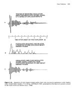
Figure 4.99: Impulse response of a temperature sensor and variation of the
associated phase values between two pulses (?τ = 0.8 µs) or four pulses (?τ
= 2.27 µs). The high degree of linearity of the measurement is striking
(reproduced by permission of Siemens AG, ZT KM, Munich)
4.3.4.2 Resonant sensors
In a reflective delay line the available path is used twice. However, if the interdigital
transducer is positioned between two fully reflective structures, then the acoustic path
can be used a much greater number of times due to multiple reflection. Such an
arrangement (see Figure 4.99) is called a surface wave one-port resonator. The
distance between the two reflectors must be an integer multiple of the half wavelength
λ
0
at the resonant frequency f
1
.

The number of wave trains stored in such a resonator will be determined by its loaded
Q factor. Normally a Q factor of 10 000 is achieved at 434 MHz and at 2.45 GHz a Q
factor of between 1500 and 3000 is reached (Reindl et al., 1998b). The displacement
of the mid-frequency ?f
1
and the displacement of the associated phase ?θ
1
of a
resonator due to a change of the physical quantity y with the loaded Q factor are
(Reindl et al., 1998a):
(4.127)
and
(4.128)
where f
1
is the unaffected resonant frequency of the resonator.
In practice, the same sensitivity is obtained as for a reflective delay line, but with a
significant reduction in chip size (Reindl et al., 1998b) (Figure 4.100).
This document was created by an unregistered ChmMagic, please go to to register it. Thanks.
Figure 4.100: Principal layout of a resonant surface wave transponder and the
associated pulse response (reproduced by permission of Siemens AG, ZT
KM, Munich)
If, instead of one resonator, several resonators with different frequencies are placed
on a crystal (Figure 4.101), then the situation is different: instead of a pulse sequence
in the time domain, such an arrangement emits a characteristic line spectrum back to
the interrogation device (Reindl et al., 1998b,c), which can be obtained from the
received sensor signal by a Fourier transformation (Figure 4.102).
Figure 4.101: Principal layout of a surface wave transponder with two
resonators of different frequency (f
1

, f
2
) (reproduced by permission of
Siemens AG, ZT KM, Munich)
Figure 4.102: Left, measured impulse response of a surface wave transponder
with two resonators of different frequency; right, after the Fourier
transformation of the impulse response the different resonant frequencies of
the two resonators are visible in the line spectrum (here— approx. 433.5 MHz
and 434 MHz) (reproduced by permission of Siemens AG, ZT KM, Munich)
The difference ?f
2-1
between the resonant frequencies of the two resonators is
determined to measure a physical quantity y in a surface wave transponder with two
resonators. Similarly to equation (4.127), this yields the following relationship (Reindl
et al., 1998c).
(4.129)
This document was created by an unregistered ChmMagic, please go to to register it. Thanks.
4.3.4.3 Impedance sensors
Using surface wave transponders, even conventional sensors can be passively
interrogated by radio if the impedance of the sensor changes as a result of the change
of a physical quantity y (e.g. photoresistor, Hall sensor, NTC or PTC resistor). To
achieve this a second interdigital transducer is used as a reflector and connected to
the external sensor (Figure 4.103). A measured quantity Ay thus changes the
terminating impedance of the additional interdigital transducer. This changes the
acoustic transmission and reflection ρ of the converter that is connected to this load,
and thus also changes the magnitude and phase of the reflected HF pulse, which can
be detected by the reader.
Figure 4.103: Principal layout of a passive surface wave transponder
connected to an external sensor (reproduced by permission of Siemens AG,
ZT KM, Munich)

4.3.5 Switched sensors
Surface wave transponders can also be passively recoded (Figure 4.104). As is the
case for an impedance sensor, a second interdigital transducer is used as a reflector.
External circuit elements of the interdigital transducer's busbar make it possible to
switch between the states 'short-circuited' and 'open'. This significantly changes the
acoustic transmission and reflection ρ of the transducer and thus also the magnitude
and phase of the reflected HF impulse that can be detected by the reader.

Figure 4.104: Passive recoding of a surface wave transponder by a switched
interdigital transducer (reproduced by permission of Siemens AG, ZT KM,
Munich)
[8]
To convert as much of the received power as possible into acoustic power, firstly the
transmission frequency f
0
of the reader should correspond with the mid-frequency of
the interdigital converter. Secondly, however, the number of transducer fingers should
This document was created by an unregistered ChmMagic, please go to to register it. Thanks.
be matched to the coupling coefficient k
2
.

This document was created by an unregistered ChmMagic, please go to to register it. Thanks.

Chapter 5: Frequency Ranges and Radio
Licensing Regulations
5.1 Frequency Ranges Used
Because RFID systems generate and radiate electromagnetic waves, they are
legally classified as radio systems. The function of other radio services must
under no circumstances be disrupted or impaired by the operation of RFID

systems. It is particularly important to ensure that RFID systems do not
interfere with nearby radio and television, mobile radio services (police, security
services, industry), marine and aeronautical radio services and mobile
telephones.
The need to exercise care with regard to other radio services significantly
restricts the range of suitable operating frequencies available to an RFID
system (Figure 5.1). For this reason, it is usually only possible to use frequency
ranges that have been reserved specifically for industrial, scientific or medical
applications. These are the frequencies classified worldwide as ISM frequency
ranges (Industrial-Scientific-Medical), and they can also be used for RFID
applications.
Figure 5.1: The frequency ranges used for RFID systems range from
the myriametric range below 135 kHz, through short wave and
ultrashort wave to the microwave range, with the highest frequency
being 24 GHz. In the frequency range above 135 kHz the ISM bands
available worldwide are preferred
In addition to ISM frequencies, the entire frequency range below 135 kHz (in
North and South America and Japan: <400 kHz) is also suitable, because it is
possible to work with high magnetic field strengths in this range, particularly
when operating inductively coupled RFID systems.
The most important frequency ranges for RFID systems are therefore 0–135
kHz, and the ISM frequencies around 6.78 (not yet available in Germany),
This document was created by an unregistered ChmMagic, please go to to register it. Thanks.
13.56 MHz, 27.125 MHz, 40.68 MHz, 433.92 MHz, 869.0 MHz, 915.0 MHz (not
in Europe), 2.45 GHz, 5.8 GHz and 24.125 GHz.
An overview of the estimated distribution of RFID transponders at the various
frequencies is shown in Figure 5.2.
Figure 5.2: The estimated distribution of the global market for
transponders over the various frequency ranges in million transponder
units (Krebs, n.d.)

5.1.1 Frequency range 9–135 kHz
The range below 135 kHz is heavily used by other radio services because it
has not been reserved as an ISM frequency range. The propagation conditions
in this long wave frequency range permit the radio services that occupy this
range to reach areas within a radius of over 1000 km continuously at a low
technical cost. Typical radio services in this frequency range are aeronautical
and marine navigational radio services (LORAN C, OMEGA, DECCA), time
signal services, and standard frequency services, plus military radio services.
Thus, in central Europe the time signal transmitter DCF 77 in Mainflingen can
be found at around the frequency 77.5 kHz. An RFID system operating at this
frequency would therefore cause the failure of all radio clocks within a radius of
several hundred metres around a reader.
In order to prevent such collisions, the future Licensing Act for Inductive Radio
Systems in Europe, 220 ZV 122, will define a protected zone of between 70
and 119 kHz, which will no longer be allocated to RFID systems.
The radio services permitted to operate within this frequency range in Germany
(source: BAPT 1997) are shown in Table 5.1.
This document was created by an unregistered ChmMagic, please go to to register it. Thanks.
Table 5.1: German radio services in the frequency range 9–135 kHz. The
actual occupation of frequencies, particularly within the range 119–135 kHz
has fallen sharply. For example, the German weather service (DWD) changed
the frequency of its weather fax transmissions to 134.2kHz as early as
mid-1996
f (kHz)ClassLocationCall
16.4FXMainflingenDMA
18.5FXBurlageDHO35
23.4FXMainflingenDMB
28.0FCBurlageDH036
36.0FCBurlageDH037
46.2FXMainflingenDCF46

47.4FCCuxhafenDHJ54
53.0FXMainflingenDCF53
55.2FXMainflingenDCF55
69.7FXKönigswusterhausenDKQ
71.4ALCoburg—
74.5FXKönigswusterhausenDKQ2
77.5TimeMainflingenDCF77
85.7ALBrilon—
87.3FXBonnDEA
87.6FXMainflingenDCF87
94.5FXKönigswusterhausenDKQ3
97.1FXMainflingenDCF97
99.7FXKönigswusterhausenDIU
100.0NLWesterland—
103.4FXMainflingenDCF23
105.0FXKönigswusterhausenDKQ4
106.2FXMainflingenDCF26
110.5FXBad VilbelDCF30
114.3ALStadtkyll—
117.4FXMainflingenDCF37
117.5FXKönigswusterhausenDKQ5
122.5DGPSMainflingenDCF42
125.0FXMainflingenDCF45
126.7ALPortens, LORAN-C, coastal —
This document was created by an unregistered ChmMagic, please go to to register it. Thanks.
f (kHz)ClassLocationCall
128.6ALZeven, DECCA, coastal
navigation
—
129.1FXMainflingen, EVU remote

control transmitter
DCF49
131.0FCKiel (military)DHJ57
131.4FXKiel (militaryDHJ57
Abbreviations: AL: Air navigation radio service, FC: Mobile marine
radio service, FX: Fixed aeronautical radio service, MS: Mobile marine
radio service, NL: Marine navigation radio service, DGPS: Differential
Global Positioning System (correction data), Time: Time signal
transmitter for 'radio clocks'.
Wire-bound carrier systems also operate at the frequencies 100 kHz, 115 kHz
and 130 kHz. These include, for example, intercom systems that use the 220 V
supply main as a transmission medium.
5.1.2 Frequency range 6.78 MHz
The range 6.765–6.795 MHz belongs to the short wave frequencies. The
propagation conditions in this frequency range only permit short ranges of up to
a few 100 km in the daytime. During the night-time hours, transcontinental
propagation is possible. This frequency range is used by a wide range of radio
services, for example broadcasting, weather and aeronautical radio services
and press agencies.
This range has not yet been passed as an ISM range in Germany, but has
been designated an ISM band by the international ITU and is being used to an
increasing degree by RFID systems (in France, among other countries).
CEPT/ERC and ETSI designate this range as a harmonised frequency in the
CEPT/ERC 70-03 regulation (see Section 5.2.1).
5.1.3 Frequency range 13.56 MHz
The range 13.553–13.567 MHz is located in the middle of the short wavelength
range. The propagation conditions in this frequency range permit
transcontinental connections throughout the day. This frequency range is used
by a wide variety of radio services (Siebel, 1983), for example press agencies
and telecommunications (PTP).

Other ISM applications that operate in this frequency range, in addition to
inductive radio systems (RFID), are remote control systems, remote controlled
models, demonstration radio equipment and pagers.
5.1.4 Frequency range 27.125 MHz
The frequency range 26.565–27.405 is allocated to CB radio across the entire
European continent as well as in the USA and Canada. Unregistered and
non-chargeable radio systems with transmit power up to 4 Watts permit radio
communication between private participants over distances of up to 30 km.
This document was created by an unregistered ChmMagic, please go to to register it. Thanks.
The ISM range between 26.957 and 27.283 MHz is located approximately in
the middle of the CB radio range. In addition to inductive radio systems (RFID),
ISM applications operating in this frequency range include diathermic
apparatus (medical application), high frequency welding equipment (industrial
application), remote controlled models and pagers.
When installing 27 MHz RFID systems for industrial applications, particular
attention should be given to any high frequency welding equipment that may be
located in the vicinity. HF welding equipment generates high field strengths,
which may interfere with the operation of RFID systems operating at the same
frequency in the vicinity. When planning 27 MHz RFID systems for hospitals
(e.g. access systems), consideration should be given to any diathermic
apparatus that may be present.
5.1.5 Frequency range 40.680 MHz
The range 40.660–40.700 MHz is located at the lower end of the VHF range.
The propagation of waves is limited to the ground wave, so damping due to
buildings and other obstacles is less marked. The frequency ranges adjoining
this ISM range are occupied by mobile commercial radio systems (forestry,
motorway management) and by television broadcasting (VHF range I).
The main ISM applications that are operated in this range are telemetry
(transmission of measuring data) and remote control applications. The author
knows of no RFID systems operating in this range, which can be attributed to

the unsuitability of this frequency range for this type of system. The ranges that
can be achieved with inductive coupling in this range are significantly lower
than those that can be achieved at all the lower frequency ranges that are
available, whereas the wavelengths of 7.5 m in this range are unsuitable for the
construction of small and cheap backscatter transponders.
5.1.6 Frequency range 433.920 MHz
The frequency range 430.000–440.000 MHz is allocated to amateur radio
services worldwide. Radio amateurs use this range for voice and data
transmission and for communication via relay radio stations or home-built
space satellites.
The propagation of waves in this UHF frequency range is approximately optical.
A strong damping and reflection of incoming electromagnetic waves occurs
when buildings and other obstacles are encountered.
Depending upon the operating method and transmission power, systems used
by radio amateurs achieve distances between 30 and 300 km. Worldwide
connections are also possible using space satellites.
The ISM range 433.050–434.790 MHz is located approximately in the middle of
the amateur radio band and is extremely heavily occupied by a wide range of
ISM applications. In addition to backscatter (RFID) systems, baby intercoms,
telemetry transmitters (including those for domestic applications, e.g. wireless
external thermometers), cordless headphones, unregistered LPD walkie-talkies
for short range radio, keyless entry systems (handheld transmitters for vehicle
central locking) and many other applications are crammed into this frequency
range. Unfortunately, mutual interference between the wide range of ISM
applications is not uncommon in this frequency range.
This document was created by an unregistered ChmMagic, please go to to register it. Thanks.
5.1.7 Frequency range 869.0 MHz
The frequency range 868–870 MHz was passed for Short Range Devices
(SRDs) in Europe at the end of 1997 and is thus available for RFID
applications in the 43 member states of CEPT.

A few Far Eastern countries are also considering passing this frequency range
for SRDs.
5.1.8 Frequency range 915.0 MHz
This frequency range is not available for ISM applications in Europe. Outside
Europe (USA and Australia) the frequency ranges 888–889 MHz and 902–928
MHz are available and are used by backscatter (RFID) systems.
Neighbouring frequency ranges are occupied primarily by D-net telephones
and cordless telephones as described in the CT1+ and CT2 standards.
5.1.9 Frequency range 2.45 GHz
The ISM range 2.400–2.4835 GHz partially overlaps with the frequency ranges
used by amateur radio and radiolocation services. The propagation conditions
for this UHF frequency range and the higher frequency SHF range are
quasi-optical. Buildings and other obstacles behave as good reflectors and
damp an electromagnetic wave very strongly at transmission (passage).
In addition to the backscatter (RFID) systems, typical ISM applications that can
be found in this frequency range are telemetry transmitters and PC LAN
systems for the wireless networking of PCs.
5.1.10 Frequency range 5.8 GHz
The ISM range 5.725–5.875 GHz partially overlaps with the frequency ranges
used by amateur radio and radiolocation services.
Typical ISM applications for this frequency range are movement sensors, which
can be used as door openers (in shops and department stores), or contactless
toilet flushing, plus backscatter (RFID) systems.
5.1.11 Frequency range 24.125 GHz
The ISM range 24.00–24.25 GHz overlaps partially with the frequency ranges
used by amateur radio and radiolocation services plus earth resources services
via satellite.
This frequency range is used primarily by movement sensors, but also
directional radio systems for data transmission. The author knows of no RFID
systems operating in this frequency range.

5.1.12 Selection of a suitable frequency for inductively coupled
RFID systems
The characteristics of the few available frequency ranges should be taken into
account when selecting a frequency for an inductively coupled RFID system.
The usable field strength in the operating range of the planned system exerts a
decisive influence on system parameters. This variable therefore deserves
This document was created by an unregistered ChmMagic, please go to to register it. Thanks.
further consideration. In addition, the bandwidth (mechanical) dimensions of the
antenna coil and the availability of the frequency band should also be
considered.
The path of field strength of a magnetic field in the near and far field was
described in detail in Section 4.2.1.1. We learned that the reduction in field
strength with increasing distance from the antenna was 60 dB/decade initially,
but that this falls to 20 dB/decade after the transition to the far field at a
distance of λ/2π. This behaviour exerts a strong influence on the usable field
strengths in the system's operating range. Regardless of the operating
frequency used, the regulation EN 300 330 specifies the maximum magnetic
field strength at a distance of 10 m from a reader (Figure 5.3).
Figure 5.3: Different permissible field strengths for inductively coupled
systems measured at a distance of 10 m (the distance specified for
licensing procedures) and the difference in the distance at which the
reduction occurs at the transition between near and far field lead to
marked differences in field strength at a distance of 1 m from the
antenna of the reader. For the field strength path at a distance under 10
cm, we have assumed that the antenna radius is the same for all
antennas
If we move from this point in the direction of the reader, then, depending upon
the wavelength, the field strength increases initially at 20 dB/decade. At an
operating frequency of 6.78 MHz the field strength begins to increase by 60
dB/decade at a distance of 7.1 m — the transition into the near field. However,

at an operating frequency of 27.125 MHz this steep increase does not begin
until a distance of 1.7 m is reached.
It is not difficult to work out that, given the same field strength at a distance of
10 m, higher usable field strengths can be achieved in the operating range of
the reader (e.g. 0–10 cm) in a lower frequency ISM band than would be the
case in a higher frequency band. At <135 kHz the relationships are even more
favourable, first because the permissible field strength limit is much higher than
it is for ISM bands above 1 MHz, and second because the 60 dB increase
takes effect immediately, because the near field in this frequency range
This document was created by an unregistered ChmMagic, please go to to register it. Thanks.
extends to at least 350m.
If we measure the range of an inductively coupled system with the same
magnetic field strength H at different frequencies we find that the range is
maximised in the frequency range around 10 MHz (Figure 5.4). This is because
of the proportionality U
ind
~ ω. At higher frequencies around 10 MHz the
efficiency of power transmission is significantly greater than at frequencies
below 135 kHz.
Figure 5.4: Transponder range at the same field strength. The induced
voltage at a transponder is measured with the antenna area and
magnetic field strength of the reader antenna held constant
(reproduced by permission of Texas Instruments)
However, this effect is compensated by the higher permissible field strength at
135 kHz, and therefore in practice the range of RFID systems is roughly the
same for both frequency ranges. At frequencies above 10 MHz the L/C
relationship of the transponder resonant circuit becomes increasingly
unfavourable, so the range in this frequency range starts to decrease.
Overall, the following preferences exist for the various frequency ranges:
< 135 kHz Preferred for large ranges and low cost

transponders.
High level of power available to the transponder.
The transponder has a low power consumption due to its
lower clock frequency.
Miniaturised transponder formats are possible (animal ID) due
to the use of ferrite coils in the transponder.
Low absorption rate or high penetration depth in non-metallic
materials and water (the high penetration depth is exploited in
animal identification by the use of the bolus, a transponder
placed in the rumen).
This document was created by an unregistered ChmMagic, please go to to register it. Thanks.
6.78 MHz Can be used for low cost and medium speed
transponders.
Worldwide ISM frequency according to ITU frequency plan;
however, this is not used in some countries (i.e. licence may
not be used worldwide).
Available power is a little greater than that for 13.56 MHz.
Only half the clock frequency of that for 13.56 MHz.
13.56 MHz Can be used for high speed/high end and medium
speed/low end applications.
Available worldwide as an ISM frequency.
Fast data transmission (typically 106 kbits/s).
High clock frequency, so cryptological functions or a
microprocessor can be realised.
Parallel capacitors for transponder coil (resonance matching)
can be realised on-chip.
27.125 MHz Only for special applications (e.g. Eurobalise)
Not a worldwide ISM frequency.
Large bandwidth, thus very fast data transmission (typically
424 kbits/s)

High clock frequency, thus cryptological functions or a
microprocessor can be realised.
Parallel capacitors for transponder coil (resonance matching)
can be realised on-chip.
Available power somewhat lower than for 13.56 MHz.
Only suitable for small ranges.

This document was created by an unregistered ChmMagic, please go to to register it. Thanks.

5.2 European Licensing Regulations
5.2.1 CEPT/ERC REC 70-03
This new CEPT harmonisation document entitled 'ERC Recommendation 70-03
relating to the use of short range devices (SRD)' (ERC, 2002) that serves as the basis
for new national regulations in all 44 member states of CEPT has been available since
October 1997. The old national regulations for Short Range Devices (SRDs) are thus
being successively replaced by a harmonised European regulation. In the new version
of February 2002 the REC 70-03 also includes comprehensive notes on national
restrictions for the specified applications and frequency ranges in the individual
member states of CEPT (REC 70-03, Appendix 3-National Restrictions). For this
reason, Section 5.3 bases its discussion of the national regulations in a CEPT member
state solely upon the example of Germany. Current notes on the regulation of short
range devices in all other CEPT members states can be found in the current version of
REC 70-03. The document is available to download on the home page of the ERO
(European Radio Office), />REC 70-03 defines frequency bands, power levels, channel spacing, and the
transmission duration (duty cycle) of short range devices. In CEPT members states
that use the R&TTE Directive (1999/5/EC), short range devices in accordance with
article 12 (CE marking) and article 7.2 (putting into service of radio equipment) can be
put into service without further licensing if they are marked with a CE mark and do not
infringe national regulatory restrictions in the member states in question (EC, 1995)
(see also Section 5.3).

REC 70-03 deals with a total of 13 different applications of short range devices at the
various frequency ranges, which are described comprehensively in its own Annexes
(Table 5.2).
Table 5.2: Short range device applications from REC 70-03
AnnexApplication
Annex 1Non-specific Short Range Devices
Annex 2Devices for Detecting Avalanche Victims
Annex 3Local Area Networks, RLANs and HIPERLANs
Annex 4Automatic Vehicle Identification for Railways (AVI)
Annex 5Road Transport and Traffic Telematics (RTTT)
Annex 6Equipment for Detecting Movement and Equipment for Alert
Annex 7Alarms
Annex 8Model Control
Annex 9Inductive Applications
Annex 10Radio Microphones
Annex 11RFID
Annex 12Ultra Low Power Active Medical Implants
Annex 13Wireless Audio Applications
REC 70-03 also refers to the harmonised ETSI standards (e.g. EN 300 330), which
This document was created by an unregistered ChmMagic, please go to to register it. Thanks.
contain measurement and testing guidelines for the licensing of radio devices.
5.2.1.1 Annex 1: Non-specific short range devices
Annex 1 describes frequency ranges and permitted transmission power for short range
devices that are not further specified (Table 5.3). These frequency ranges can
expressly also be used by RFID systems, if the specified levels and powers are
adhered to.
Table 5.3: Non-specific short range devices
Frequency bandPowerComment
6785–6795 kHz
42 dBµA/m @ 10

m

13.553–13.567 MHz
42 dBµA/m @ 10
m

26.957–27.283 MHz
42 dBµA/m
(10 mW ERP)
40.660–40.700 MHz10 mW ERP

138.2–138.45 MHz10 mW ERPOnly available in some
states
433.050–434.790 MHz10 mW ERP<10% duty cycle
433.050–434.790 MHz1 mW ERPUp to 100% duty cycle
868.000–868.600 MHz25 mW ERP<1% duty cycle
868.700–869.200 MHz25 mW ERP<0.1% duty cycle
869.300–869.400 MHz10 mW ERP

869.400-860.650 MHz500 mW ERP<10% duty cycle
869.700–870.000 MHz5 mW ERP

2400–2483.5 MHz10 mW EIRP

5725–5875 MHz25 mW EIRP

24.00–24.25 GHz100 mW

61.0–61.5100 mW EIRP

122–123 GHz100 mW EIRP

244–246 GHz10 mW EIRP

Relevant harmonised standards: EN 300 220, EN 300 330, EN 300 440.
5.2.1.2 Annex 4: Railway applications
Annex 4 describes frequency ranges and permitted transmission power for short range
devices in application for rail traffic applications. RFID transponder systems such as
the Eurobalise S21 (see Section 13.5.1) or vehicle identification by transponder (see
Section 13.5.2) are among these applications.
This document was created by an unregistered ChmMagic, please go to to register it. Thanks.
Table 5.4: Railway applications
Frequency bandPowerComment
4515 kHz
7 dB µA/m @ 10
m
Euroloop (spectrum mask
available)
27.095 MHz
42 dB µA/mEurobalise (5 dBµA/m @ ±200
kHz
2446–2454 MHz500 mW EIRPTransponder applications (AVI)
Relevant harmonised standards: EN 300 761, EN 300 330.
Table 5.5: Road Transport and Traffic Telematics (RTTT)
Frequency bandPowerComment
5795–5815 MHz8 W EIRPRoad toll systems
63–64 GHzt.b.d.Vehicle — vehicle communication
76–77 GHz55 dBm peakVehicle — radar systems
Relevant harmonised standards: EN 300 674, EN 301 091, EN 201 674.
Table 5.6: Inductive applications

Frequency bandPowerComment
9.000–59.750 kHzSee comment
72 dBµ A/m at 30 kHz,
60.250–70.000 kHz

descending by -3dB/Ok
119–135 kHz

59.750–60.250 kHz
42 dB µA/m @ 10 m

70–119 kHz

6765–6795 kHz
42 dB µA/m @ 10 m

7400–8800 kHz
9 dB µA/m
EAS systems
13.553–13.567 MHz
42 dB µA/m @ 10 m(9 dBµA/m @ ± 150 kHz)
26.957–27.283 MHz
42 dB µA/m @ 10 m(9 dBµA/m @ ± 150 kHz)
Relevant harmonised standards: EN 300 330.
Table 5.7: RFID applications
Frequency bandPowerComment
2446–2454 MHz500 mW EIRP
4W EIRP
100% duty cycle
<15% duty cycle; only within buildings

Relevant harmonised standards: EN 300 440.
This document was created by an unregistered ChmMagic, please go to to register it. Thanks.
Table 5.8: Proposal for a further frequency range for RFID systems
Frequency bandPowerComment
865.0–868.0
MHz:

Channels with 100 kHz channel
spacing
865.0–865.6 MHz100 mW
EIRP

865.6–867.6 MHz2 W EIRP

867.6–868.0 MHz
100 mW
EIRP

5.2.1.3 Annex 5: Road transport and traffic telematics
Annex 5 describes frequency ranges and permitted transmission power for short range
devices in traffic telematics and vehicle identification applications. These applications
include the use of RFID transponders in road toll systems.
5.2.1.4 Annex 9: Inductive applications
Annex 9 describes frequency ranges and permitted transmission power for inductive
radio systems. These include RFID transponders and Electronic Article Surveillance
(EAS) in shops.
5.2.1.5 Annex 11: RFID applications
Annex 11 describes the frequency ranges and permitted transmission power for RFID
systems. An 8 MHz segment of the 2.45 GHz frequency band is cleared for operation
at an increased transmission power.

5.2.1.6 Frequency range 868 MHz
The subject of possible future frequency ranges and transmission power for RFID
systems in the 868 MHz range is currently under discussion by the European
Radiocommunications Committee (ERC). In addition to the frequency range
869.4-869.65 MHz (500 mW EIRP at 10% duty cycle, Annex 1) that is already
available, a future frequency range is being considered for RFID systems. A final
decision is still awaited from the ERC.
5.2.2 EN 300 330: 9 kHz-25 MHz
The standards drawn up by ETSI (European Telecommunications Standards Institute)
serve to provide the national telecommunications authorities with a basis for the
creation of national regulations for the administration of radio and telecommunications.
The ETSI EN 300 330 standard forms the basis for European licensing regulations for
inductive radio system:
ETSI EN 300 330: 'Electromagnetic compatibility and Radio spectrum
Matters (ERM); Short Range Devices (SRD); Radio equipment in the
frequency range 9 kHz to 25 MHz and inductive loop systems in the
frequency range 9 kHz to 30 MHz'.
Part 1: 'Technical characteristics and test methods'
Part 2: 'Harmonized EN under article 3.2 of the R&TTE Directive'
In addition to inductive radio systems, EN 300330 also deals with Electronic Article
Surveillance (for shops), alarm systems, telemetry transmitters, and short range
telecontrol systems, which are considered under the collective term Short Range
This document was created by an unregistered ChmMagic, please go to to register it. Thanks.
Devices (SRDs).
In addition to the CEPT member states, this regulation is also used by many Asiatic
and American states in the licensing of RFID systems.
EN 3003300 thus primarily defines measurement procedures for transmitter and
receiver that can be used to reproducibly verify adherence to the prescribed limit
values in relation to ERC REC 70-03.
Inductive loop coil transmitters in accordance with EN 300330 are characterised by the

fact that the antenna is formed by a loop of wire with one or more windings. EN
300330 differentiates between four product classes (Table 5.9).
Table 5.9: Classification of the product types
Class
1
Transmitter with inductive loop antenna, in which the antenna is
integrated into the device or permanently connected to it. Enclosed
antenna area <30 m
2
.
Class
2
Transmitter with inductive loop antenna, in which the antenna is
manufactured to the customer's requirements. Devices belonging to
class 2, like class 1 devices, are tested using two typical
customer-specific antennas. The enclosed antenna area must be
less than 30 m
2
.
Class
3
Transmitter with large inductive loop antenna, >30 m
2
antenna
area. Class 3 devices are tested without an antenna.
Class
4
E field transmitter. These devices are tested with an antenna.
All the inductively coupled RFID systems in the frequency range 9 kHz–30 MHz
described in EN 300 330 belong to the class 1 and class 2 types. Therefore class 3

and class 4 types will not be further considered in this book.
5.2.2.1 Carrier power - limit values for H field transmitters
In class 1 and class 2 inductive loop coil transmitters (integral antenna) the H field of
the radio system is measured in the direction in which the field strength reaches a
maximum. The measurement should be performed in free space, with a distance of
10m between measuring antenna and measurement object. The transmitter is not
modulated during the field strength measurement.
The limit values listed in Table 5.10 have been defined. See Figure 5.5.
This document was created by an unregistered ChmMagic, please go to to register it. Thanks.
Table 5.10: Maximum permitted magnetic field strength at a distance of 10m
Frequency range
(MHz)
Maximum H field at a distance of 10 m
0.009–0.030
72 dBµA/m
0.030–0.070
72 dBµA/m at 0.030 MHz descending by -3
dB/octave
0.05975–0.06025
42 dBµA/m
0.070–0.119

0.119–0.135
72 dBµA/m at 0.03 MHz, descending by -3dB/oct
0.135–1.0
37.7 dBµA/m at 0.135 MHz, descending by -3
dB/octave
1.0–4.642
29 dBµA/m at 1.0 MHz, descending by -9
dB/octave

4.643–30
9 dBµA/m
6.675–6.795
42 dBµA/m
13.553–13.567

25.957–27.283


Figure 5.5: Limit values for the magnetic field strength H measured at a
distance of 10 m, according to Table 5.10
In loop antennas with an antenna area between 0.05 m
2
(diameter 24 cm) and 0.16
m
2
(diameter 44 cm) a correction factor must be subtracted from the values in Table
5.10. The following is true:
(5.1)
For a typical RFID antenna with a diameter of 32 cm there would be a correction factor
of -3 dB and thus at 13.56 MHz the maximum field strength would be 39 dBµ V/m at a
distance of 10 m.
This document was created by an unregistered ChmMagic, please go to to register it. Thanks.