rfid handbook fundamentals and applications in contactless smart cards and identification second edition phần 10 pdf

List of Figures
Chapter 1: Introduction
Figure 1.1: The estimated growth of the global market for RFID
systems between 2000 and 2005 in million $US, classified by
application
Figure 1.2: Overview of the most important auto-ID procedures
Figure 1.3: Example of the structure of a barcode in EAN coding
Figure 1.4: This barcode is printed on the back of this book and
contains the ISBN number of the book
Figure 1.5: Typical architecture of a memory card with security logic
Figure 1.6: Typical architecture of a microprocessor card
Figure 1.7: The reader and transponder are the main components of
every RFID system
Figure 1.8: RFID reader and contactless smart card in practical use
(reproduced by permission of Kaba Benzing GmbH)
Figure 1.9: Basic layout of the RFID data-carrying device, the
transponder. Left, inductively coupled transponder with antenna coil;
right, microwave transponder with dipolar antenna
Chapter 2: Differentiation Features of RFID
Systems
Figure 2.1: The various features of RFID systems (Integrated Silicon
Design, 1996)
Figure 2.2: Different construction formats of disk transponders. Right,
transponder coil and chip prior to fitting in housing; left, different
construction formats of reader antennas (reproduced by permission of
Deister Electronic, Barsinghausen)
Figure 2.3: Close-up of a 32 mm glass transponder for the identification
of animals or further processing into other construction formats
(reproduced by permission of Texas Instruments)
Figure 2.4: Mechanical layout of a glass transponder

Figure 2.5: Transponder in a plastic housing (reproduced by permission
of Philips Electronics B.V.)
Figure 2.6: Mechanical layout of a transponder in a plastic housing.
The housing is just 3 mm thick
Figure 2.7: Transponder in a standardised construction format in
accordance with ISO 69873, for fitting into one of the retention knobs of
This document was created by an unregistered ChmMagic, please go to to register it. Thanks.
a CNC tool (reproduced by permission of Leitz GmbH & Co.,
Oberkochen)
Figure 2.8: Mechanical layout of a transponder for fitting into metal
surfaces. The transponder coil is wound around a U-shaped ferrite
core and then cast into a plastic shell. It is installed with the opening of
the U-shaped core uppermost
Figure 2.9: Keyring transponder for an access system (reproduced by
permission of Intermarketing)
Figure 2.10: Watch with integral transponder in use in a contactless
access authorisation system (reproduced by permission of Junghans
Uhren GmbH, Schramberg)
Figure 2.11: Layout of a contactless smart card— card body with
transponder module and antenna
Figure 2.12: Semitransparent contactless smart card. The transponder
antenna can be clearly seen along the edge of the card (reproduced by
permission of Giesecke & Devrient, Munich)
Figure 2.13: Microwave transponders in plastic shell housings
(reproduced by permission of Pepperl & Fuchs GmbH)
Figure 2.14: Smart label transponders are thin and flexible enough to
be attached to luggage in the form of a self-adhesive label (reproduced
by permission of i-code-Transponder, Philips Semiconductors,
A-Gratkorn)
Figure 2.15: A smart label primarily consists of a thin paper or plastic

foil onto which the transponder coil and transponder chip can be
applied (Tag-It Transponder, reproduced by permission of Texas
Instruments, Friesing)
Figure 2.16: Extreme miniaturisation of transponders is possible using
coil-on-chip technology (reproduced by permission of Micro Sensys,
Erfurt)
Figure 2.17: RFID systems can be classified into low-end and high-end
systems according to their functionality
Figure 2.18: Comparison of the relative interrogation zones of different
systems
Chapter 3: Fundamental Operating Principles
Figure 3.1: The allocation of the different operating principles of RFID
systems into the sections of the chapter
Figure 3.2: Operating principle of the EAS radio frequency procedure
Figure 3.3: The occurrence of an impedance 'dip' at the generator coil
at the resonant frequency of the security element (Q = 90, k = 1%). The
generator frequency f
G
is continuously swept between two cut-off
frequencies. An RF tag in the generator field generates a clear dip at
its resonant frequency f
R
This document was created by an unregistered ChmMagic, please go to to register it. Thanks.
Figure 3.4: Left, typical frame antenna of an RF system (height
1.20–1.60 m); right, tag designs
Figure 3.5: Basic circuit and typical construction format of a microwave
tag
Figure 3.6: Microwave tag in the interrogation zone of a detector
Figure 3.7: Basic circuit diagram of the EAS frequency division
procedure— security tag (transponder) and detector (evaluation

device)
Figure 3.8: Left, typical antenna design for a security system (height
approximately 1.40m); right, possible tag designs
Figure 3.9: Electromagnetic labels in use (reproduced by permission of
Schreiner Codedruck, Munich)
Figure 3.10: Practical design of an antenna for an article surveillance
system (reproduced by permission of METO EAS System 2200,
Esselte Meto, Hirschborn)
Figure 3.11: Acoustomagnetic system comprising transmitter and
detection device (receiver). If a security element is within the field of the
generator coil this oscillates like a tuning fork in time with the pulses of
the generator coil. The transient characteristics can be detected by an
analysing unit
Figure 3.12: Representation of full duplex, half duplex and sequential
systems over time. Data transfer from the reader to the transponder is
termed downlink, while data transfer from the transponder to the reader
is termed uplink
Figure 3.13: Power supply to an inductively coupled transponder from
the energy of the magnetic alternating field generated by the reader
Figure 3.14: Different designs of inductively coupled transponders. The
photo shows half finished transponders, i.e. transponders before
injection into a plastic housing (reproduced by permission of AmaTech
GmbH & Co. KG, D-Pfronten)
Figure 3.15: Reader for inductively coupled transponder in the
frequency range <135 kHz with integral antenna (reproduced by
permission of easy-key System, micron, Halbergmoos)
Figure 3.16: Generation of load modulation in the transponder by
switching the drain-source resistance of an FET on the chip. The
reader illustrated is designed for the detection of a subcarrier
Figure 3.17: Load modulation creates two sidebands at a distance of

the subcarrier frequency f
S
around the transmission frequency of the
reader. The actual information is carried in the sidebands of the two
subcarrier sidebands, which are themselves created by the modulation
of the subcarrier
Figure 3.18: Example circuit for the generation of load modulation with
subcarrier in an inductively coupled transponder
Figure 3.19: Basic circuit of a transponder with subharmonic back
frequency. The received clocking signal is split into two, the data is
This document was created by an unregistered ChmMagic, please go to to register it. Thanks.
modulated and fed into the transponder coil via a tap
Figure 3.20: Active transponder for the frequency range 2.45 GHz. The
data carrier is supplied with power by two lithium batteries. The
transponder's microwave antenna is visible on the printed circuit board
in the form of a u-shaped area (reproduced by permission of Pepperl &
Fuchs, Mannheim)
Figure 3.21: Operating principle of a backscatter transponder. The
impedance of the chip is 'modulated' by switching the chip's FET
(Integrated Silicon Design, 1996)
Figure 3.22: Close coupling transponder in an insertion reader with
magnetic coupling coils
Figure 3.23: Capacitive coupling in close coupling systems occurs
between two parallel metal surfaces positioned a short distance apart
from each other
Figure 3.24: An electrically coupled system uses electrical
(electrostatic) fields for the transmission of energy and data
Figure 3.25: Necessary electrode voltage for the reading of a
transponder with the electrode size a × b = 4.5 cm × 7 cm (format
corresponds with a smart card), at a distance of 1 m (f = 125 kHz)

Figure 3.26: Equivalent circuit diagram of an electrically coupled RFID
system
Figure 3.27: Comparison of induced transponder voltage in FDX/HDX
and SEQ systems (Schürmann, 1993)
Figure 3.28: Block diagram of a sequential transponder by Texas
Instruments TIRIS® Systems, using inductive coupling
Figure 3.29: Voltage path of the charging capacitor of an inductively
coupled SEQ transponder during operation
Figure 3.30: Basic layout of an SAW transponder. Interdigital
transducers and reflectors are positioned on the piezoelectric crystal
Figure 3.31: Surface acoustic wave transponder for the frequency
range 2.45 GHz with antenna in the form of microstrip line. The
piezocrystal itself is located in an additional metal housing to protect it
against environmental influences (reproduced by permission of
Siemens AG, ZT KM, Munich)
Chapter 4: Physical Principles of RFID Systems
Figure 4.1: Lines of magnetic flux are generated around every
current-carrying conductor
Figure 4.2: Lines of magnetic flux around a current-carrying conductor
and a current-carrying cylindrical coil
Figure 4.3: The path of the lines of magnetic flux around a short
cylindrical coil, or conductor loop, similar to those employed in the
transmitter antennas of inductively coupled RFID systems
This document was created by an unregistered ChmMagic, please go to to register it. Thanks.
Figure 4.4: Path of magnetic field strength H in the near field of short
cylinder coils, or conductor coils, as the distance in the x direction is
increased
Figure 4.5: Field strength H of a transmission antenna given a constant
distance x and variable radius R, where I = 1 A and N = 1
Figure 4.6: Relationship between magnetic flux Φ and flux density B

Figure 4.7: Definition of inductance L
Figure 4.8: The definition of mutual inductance M
21
by the coupling of
two coils via a partial magnetic flow
Figure 4.9: Graph of mutual inductance between reader and
transponder antenna as the distance in the x direction increases
Figure 4.10: Graph of the coupling coefficient for different sized
conductor loops. Transponder antenna— r
Transp
= 2 cm, reader
antenna— r
1
= 10 cm, r
2
= 7.5 cm, r
3
= 1 cm
Figure 4.11: Induced electric field strength E in different materials.
From top to bottom— metal surface, conductor loop and vacuum
Figure 4.12: Left, magnetically coupled conductor loops; right,
equivalent circuit diagram for magnetically coupled conductor loops
Figure 4.13: Equivalent circuit diagram for magnetically coupled
conductor loops. Transponder coil L
2
and parallel capacitor C
2
form a
parallel resonant circuit to improve the efficiency of voltage transfer.
The transponder's data carrier is represented by the grey box

Figure 4.14: Plot of voltage at a transponder coil in the frequency range
1 to 100 MHz, given a constant magnetic field strength H or constant
current i
1
. A transponder coil with a parallel capacitor shows a clear
voltage step-up when excited at its resonant frequency ( f
RES
= 13.56
MHz)
Figure 4.15: Plot of voltage u
2
for different values of transponder
inductance L
2
. The resonant frequency of the transponder is equal to
the transmission frequency of the reader for all values of L
2
(i
1
= 0.5 A,
f = 13.56 MHz, R
2
= 1 O)
Figure 4.16: Graph of the Q factor as a function of transponder
inductance L
2
, where the resonant frequency of the transponder is
constant (f = 13.56 MHz, R
2
= 1O)

Figure 4.17: Operating principle for voltage regulation in the
transponder using a shunt regulator
Figure 4.18: Example of the path of voltage u
2
with and without shunt
regulation in the transponder, where the coupling coefficient k is varied
by altering the distance between transponder and reader antenna.
(The calculation is based upon the following parameters— i
1
= 0.5 A,
L
1
= 1 µH, L
2
= 3.5 µH, R
L
= 2kO, C
2
= 1/ω
2
L
2
)
Figure 4.19: The value of the shunt resistor R
S
must be adjustable over
a wide range to keep voltage u
2
constant regardless of the coupling
This document was created by an unregistered ChmMagic, please go to to register it. Thanks.

coefficient k (parameters as Figure 4.18)
Figure 4.20: Example circuit for a simple shunt regulator
Figure 4.21: Interrogation sensitivity of a contactless smart card where
the transponder resonant frequency is detuned in the range 10–20
MHz (N = 4, A = 0.05 × 0.08 m
2
, u
2
= 5V, L
2
= 3.5 µH, R
2
= 5O, R
L
=
1.5 kO). If the transponder resonant frequency deviates from the
transmission frequency (13.56 MHz) of the reader an increasingly high
field strength is required to address the transponder. In practical
operation this results in a reduction of the read range
Figure 4.22: The energy range of a transponder also depends upon the
power consumption of the data carrier (R
L
). The transmitter antenna of
the simulated system generates a field strength of 0.115 A/m at a
distance of 80 cm, a value typical for RFID systems in accordance with
ISO 15693 (transmitter— I = 1A, N
1
= 1, R = 0.4m. Transponder— A =
0.048 × 0.076m
2

(smart card), N = 4, L
2
= 3.6 µH, u
2min
= 5V/3V)
Figure 4.23: Cross-section through reader and transponder antennas.
The transponder antenna is tilted at an angle ϑ in relation to the reader
antenna
Figure 4.24: Interrogation zone of a reader at different alignments of
the transponder coil
Figure 4.25: Equivalent circuit diagram of a reader with antenna L
1
.
The transmitter output branch of the reader generates the HF voltage
u
0
. The receiver of the reader is directly connected to the antenna coil
L
1
Figure 4.26: Voltage step-up at the coil and capacitor in a series
resonant circuit in the frequency range 10–17 MHz (f
RES
= 13.56 MHz,
u
0
= 10V(!), R
1
= 2.5 O, L
1
= 2µH, C

1
= 68.8 pF). The voltage at the
conductor coil and series capacitor reaches a maximum of above 700
V at the resonant frequency. Because the resonant frequency of the
reader antenna of an inductively coupled system always corresponds
with the transmission frequency of the reader, components should be
sufficiently voltage resistant
Figure 4.27: Equivalent circuit diagram of the series resonant circuit —
the change in current i
1
in the conductor loop of the transmitter due to
the influence of a magnetically coupled transponder is represented by
the impedance
Figure 4.28: The vector diagram for voltages in the series resonance
circuit of the reader antenna at resonant frequency. The figures for
individual voltages u
L1
and u
C1
can reach much higher levels than the
total voltage u
0
Figure 4.29: Simple equivalent circuit diagram of a transponder in the
vicinity of a reader. The impedance Z
2
of the transponder is made up of
the load resistor R
L
(data carrier) and the capacitor C
2

Figure 4.30: The impedance locus curve of the complex transformed
This document was created by an unregistered ChmMagic, please go to to register it. Thanks.
transponder impedance as a function of transmission frequency
(f
TX
= 1–30 MHz) of the reader corresponds with the impedance locus
curve of a parallel resonant circuit
Figure 4.31: The equivalent circuit diagram of complex transformed
transponder impedance is a damped parallel resonant circuit
Figure 4.32: The locus curve of (k = 0–1) in the complex
impedance plane as a function of the coupling coefficient k is a straight
line
Figure 4.33: The locus curve of (C
2
= 10–110 pF) in the complex
impedance plane as a function of the capacitance C
2
in the
transponder is a circle in the complex Z plane. The diameter of the
circle is proportional to k
2
Figure 4.34: Value and phase of the transformed transponder
impedance as a function of C
2
. The maximum value of is
reached when the transponder resonant frequency matches the
transmission frequency of the reader. The polarity of the phase angle
of varies
Figure 4.35: Locus curve of (R
L

= 0.3–3 kO) in the impedance
plane as a function of the load resistance R
L
in the transponder at
different transponder resonant frequencies
Figure 4.36: The value of as a function of the transponder
inductance L
2
at a constant resonant frequency f
RES
of the
transponder. The maximum value of coincides with the
maximum value of the Q factor in the transponder
Figure 4.37: Equivalent circuit diagram for a transponder with load
modulator. Switch S is closed in time with the data stream — or a
modulated subcarrier signal — for the transmission of data
Figure 4.38: Locus curve of the transformed transponder impedance
with ohmic load modulation (R
L
||R
mod
= 1.5-5kO) of an inductively
coupled transponder. The parallel connection of the modulation resistor
R
mod
results in a lower value of
Figure 4.39: Vector diagram for the total voltage u
RX
that is available to
the receiver of a reader. The magnitude and phase of u

RX
are
modulated at the antenna coil of the reader (L
1
) by an ohmic load
modulator
Figure 4.40: Equivalent circuit diagram for a transponder with
capacitive load modulator. To transmit data the switch S is closed in
time with the data stream — or a modulated subcarrier signal
This document was created by an unregistered ChmMagic, please go to to register it. Thanks.
Figure 4.41: Locus curve of transformed transponder impedance for the
capacitive load modulation (C
2
||C
mod
= 40–60 pF) of an inductively
coupled transponder. The parallel connection of a modulation capacitor
C
mod
results in a modulation of the magnitude and phase of the
transformed transponder impedance
Figure 4.42: Vector diagram of the total voltage u
RX
available to the
receiver of the reader. The magnitude and phase of this voltage are
modulated at the antenna coil of the reader (L
1
) by a capacitive load
modulator
Figure 4.43: The transformed transponder impedance reaches a peak

at the resonant frequency of the transponder. The amplitude of the
modulation sidebands of the current i
2
is damped due to the influence
of the bandwidth B of the transponder resonant circuit (where f
H
= 440
kHz, Q = 30)
Figure 4.44: If the transponder resonant frequency is markedly detuned
compared to the transmission frequency of the reader the two
modulation sidebands will be transmitted at different levels. (Example
based upon subcarrier frequency f
H
= 847 kHz)
Figure 4.45: Measurement circuit for the measurement of the magnetic
coupling coefficient k. N1— TL081 or LF 356N, R1— 100–500 O
(reproduced by permission of TEMIC Semiconductor GmbH,
Heilbronn)
Figure 4.46: Equivalent circuit diagram of the test transponder coil with
the parasitic capacitances of the measuring circuit
Figure 4.47: The circuit for the measurement of the transponder
resonant frequency consists of a coupling coil L
1
and a measuring
device that can precisely measure the complex impedance of Z
1
over a
certain frequency range
Figure 4.48: The measurement of impedance and phase at the
measuring coil permits no conclusion to be drawn regarding the

frequency of the transponder
Figure 4.49: The locus curve of impedance Z
1
in the frequency range
1–30 MHz
Figure 4.50: Typical magnetisation or hysteresis curve for a
ferromagnetic material
Figure 4.51: Configuration of a ferrite antenna in a 135 kHz glass
transponder
Figure 4.52: Reader antenna (left) and gas bottle transponder in a
u-shaped core with read head (right) can be mounted directly upon or
within metal surfaces using ferrite shielding
Figure 4.53: Right, fitting a glass transponder into a metal surface; left,
the use of a thin dielectric gap allows the transponders to be read even
through a metal casing (Photo— HANEX HXID system with Sokymat
glass transponder in metal, reproduced by permission of HANEX Co.
Ltd, Japan)
This document was created by an unregistered ChmMagic, please go to to register it. Thanks.
Figure 4.54: Path of field lines around a transponder encapsulated in
metal. As a result of the dielectric gap the field lines run in parallel to
the metal surface, so that eddy current losses are kept low (reproduced
by permission of HANEX Co. Ltd, Japan)
Figure 4.55: Cross-section through a sandwich made of disk
transponder and metal plates. Foils made of amorphous metal cause
the magnetic field lines to be directed outwards
Figure 4.56: The creation of an electromagnetic wave at a dipole
antenna. The electric field E is shown. The magnetic field H forms as a
ring around the antenna and thus lies at right angles to the electric field
Figure 4.57: Graph of the magnetic field strength H in the transition
from near to far field at a frequency of 13.56 MHz

Figure 4.58: The Poynting radiation vector S as the vector product of E
and H
Figure 4.59: Definition of the polarisation of electromagnetic waves
Figure 4.60: Reflection off a distant object is also used in radar
technology
Figure 4.61: Propagation of waves emitted and reflected at the
transponder
Figure 4.62: Radiation pattern of a dipole antenna in comparison to the
radiation pattern of an isotropic emitter
Figure 4.63: Equivalent circuit of an antenna with a connected
transponder
Figure 4.64: Relationship between the radiation density S and the
received power P of an antenna
Figure 4.65: Graph of the relative effective aperture A
e
and the relative
scatter aperture σ in relation to the ratio of the resistances R
A
and R
r
.
Where R
T
/R
A
= 1 the antenna is operated using power matching (R
T
=
R
r

). The case R
T
/R
A
= 0 represents a short-circuit at the terminals of
the antenna
Figure 4.66: 915 MHz transponder with a simple, extended dipole
antenna. The transponder can be seen half way along (reproduced by
permission of Trolleyscan, South Africa)
Figure 4.67: Different dipole antenna designs — from top to bottom—
simple extended dipole, 2-wire folded dipole, 3-wire folded dipole
Figure 4.68: Typical design of a Yagi-Uda directional antenna (six
elements), comprising a driven emitter (second transverse rod from
left), a reflector (first transverse rod from left) and four directors (third to
sixth transverse rods from left) (reproduced by permission of
Trolleyscan, South Africa)
Figure 4.69: Fundamental layout of a patch antenna. The ratio of L
p
to
h
D
is not shown to scale
Figure 4.70: Practical layout of a patch antenna for 915 MHz on a
This document was created by an unregistered ChmMagic, please go to to register it. Thanks.
printed circuit board made of epoxy resin (reproduced by permission of
Trolleyscan, South Africa)
Figure 4.71: Supply of a λ/2 emitter quad of a patch antenna via the
supply line on the reverse
Figure 4.72: The interconnection of patch elements to form a group
increases the directional effect and gain of the antenna

Figure 4.73: Layout of a slot antenna for the UHF and microwave range
Figure 4.74: Model of a microwave RFID system when a transponder is
located in the interrogation zone of a reader. The figure shows the flow
of HF power throughout the entire system
Figure 4.75: Functional equivalent circuit of the main circuit
components of a microwave transponder (left) and the simplified
equivalent circuit (right)
Figure 4.76: The maximum power P
e
(0 dBm = 1 mW) available for the
operation of the transponder, in the case of power matching at the
distance r, using a dipole antenna at the transponder
Figure 4.77: A Schottky diode is created by a metal-semiconductor
junction. In small signal operation a Schottky diode can be represented
by a linear equivalent circuit
Figure 4.78: (a) Circuit of a Schottky detector with impedance
transformation for power matching at the voltage source and (b) the HF
equivalent circuit of the Schottky detector
Figure 4.79: When operated at powers below -20 dBm (10 µW) the
Schottky diode is in the square law range
Figure 4.80: Circuit of a Schottky detector in a voltage doubler circuit
(villard-rectifier)
Figure 4.81: Output voltage of a Schottky detector in a voltage doubler
circuit. In the input power range -20 to -10 dBm the transition from
square law to linear law detection can be clearly seen (R
L
= 500 kO, I
s
= 2 µA, n = 1.12)
Figure 4.82: The factor M describes the influence of the parasitic

junction capacitance C
j
upon the output voltage u
chip
at different
frequencies. As the junction resistance R
j
falls, the influence of the
junction capacitance C
j
also declines markedly. Markers at 868 MHz
and 2.45 GHz
Figure 4.83: Voltage sensitivity γ2 of a Schottky detector in relation to
the total current I
T
· C
j
= 0.25 pF, R
S
= 25 O, R
L
= 100 kO
Figure 4.84: Matching of a Schottky detector (point 1) to a dipole
antenna (point 4) by means of the series connection of a coil (point
1-2), the parallel connection of a second coil (point 2–3), and finally the
series connection of a capacitor (point 3–4)
Figure 4.85: By suitable design of the transponder antenna the
impedance of the antenna can be designed to be the complex
conjugate of the input impedance of the transponder chip (reproduced
This document was created by an unregistered ChmMagic, please go to to register it. Thanks.

by permission of Rafsec, Palomar-Konsortium,
PALOMAR-Transponder)
Figure 4.86: The superposition of the field originally emitted with
reflections from the environment leads to local cancellations. x axis,
distance from reader antenna; y axis, path attenuation in decibels
(reproduced by permission of Rafsec, Palomar-Konsortium)
Figure 4.87: Generation of the modulated backscatter by the
modulation of the transponder impedance Z
T
(= R
T
)
Figure 4.88: Block diagram of a passive UHF transponder (reproduced
by permission of Rafsec, Palomar-Konsortium, PALOMAR
Transponder)
Figure 4.89: Example of the level relationships in a reader. The noise
level at the receiver of the reader lies around 100 dB below the signal
of the carrier. The modulation sidebands of the transponder can clearly
be seen. The reflected carrier signal cannot be seen, since the level of
the carrier signal of the reader's transmitter, which is the same
frequency, is higher by orders of magnitude
Figure 4.90: Damping of a signal on the way to and from the
transponder
Figure 4.91: The section through a crystal shows the surface distortions
of a surface wave propagating in the z-direction (reproduced by
permission of Siemens AG, ZT KM, Munich)
Figure 4.92: Principal structure of an interdigital transducer. Left,
arrangement of the finger-shaped electrodes of an interdigital
transducer; right, the creation of an electric field between electrodes of
different polarity (reproduced by permission of Siemens AG, ZT KM,

Munich)
Figure 4.93: Scanning electron microscope photograph of several
surface wave packets on a piezoelectric crystal. The interdigital
transducer itself can be seen to the bottom left of the picture. An
electric alternating voltage at the electrodes of the interdigital
transducer generates a surface wave in the crystal lattice as a result of
the piezoelectric effect. Conversely, an incoming surface wave
generates an electric alternating voltage of the same frequency at the
electrodes of the transducer (reproduced by permission of Siemens
AG, ZT KM, Munich)
Figure 4.94: Geometry of a simple reflector for surface waves
(reproduced by permission of Siemens AG, ZT KM, Munich)
Figure 4.95: Functional diagram of a surface wave transponder
(reproduced by permission of Siemens AG, ZT KM, Munich)
Figure 4.96: Sensor echoes from the surface wave transponder do not
arrive until environmental echoes have decayed (reproduced by
permission of Siemens AG, ZT KM, Munich)
Figure 4.97: Surface wave transponders operate at a defined phase in
relation to the interrogation pulse. Left, interrogation pulse, consisting of
four individual pulses; right, the phase position of the response pulse,
shown in a clockface diagram, is precisely defined (reproduced by
This document was created by an unregistered ChmMagic, please go to to register it. Thanks.
permission of Siemens AG, ZT KM, Munich)
Figure 4.98: Calculation of the system range of a surface wave
transponder system in relation to the integration time t
i
at different
frequencies (reproduced by permission of Siemens AG, ZT KM,
Munich)
Figure 4.99: Impulse response of a temperature sensor and variation of

the associated phase values between two pulses (?τ = 0.8 µs) or four
pulses (?τ = 2.27 µs). The high degree of linearity of the measurement
is striking (reproduced by permission of Siemens AG, ZT KM, Munich)
Figure 4.100: Principal layout of a resonant surface wave transponder
and the associated pulse response (reproduced by permission of
Siemens AG, ZT KM, Munich)
Figure 4.101: Principal layout of a surface wave transponder with two
resonators of different frequency (f
1
, f
2
) (reproduced by permission of
Siemens AG, ZT KM, Munich)
Figure 4.102: Left, measured impulse response of a surface wave
transponder with two resonators of different frequency; right, after the
Fourier transformation of the impulse response the different resonant
frequencies of the two resonators are visible in the line spectrum
(here— approx. 433.5 MHz and 434 MHz) (reproduced by permission
of Siemens AG, ZT KM, Munich)
Figure 4.103: Principal layout of a passive surface wave transponder
connected to an external sensor (reproduced by permission of
Siemens AG, ZT KM, Munich)
Figure 4.104: Passive recoding of a surface wave transponder by a
switched interdigital transducer (reproduced by permission of Siemens
AG, ZT KM, Munich)
Chapter 5: Frequency Ranges and Radio
Licensing Regulations
Figure 5.1: The frequency ranges used for RFID systems range from
the myriametric range below 135 kHz, through short wave and
ultrashort wave to the microwave range, with the highest frequency

being 24 GHz. In the frequency range above 135 kHz the ISM bands
available worldwide are preferred
Figure 5.2: The estimated distribution of the global market for
transponders over the various frequency ranges in million transponder
units (Krebs, n.d.)
Figure 5.3: Different permissible field strengths for inductively coupled
systems measured at a distance of 10 m (the distance specified for
licensing procedures) and the difference in the distance at which the
reduction occurs at the transition between near and far field lead to
marked differences in field strength at a distance of 1 m from the
antenna of the reader. For the field strength path at a distance under
10 cm, we have assumed that the antenna radius is the same for all
antennas
This document was created by an unregistered ChmMagic, please go to to register it. Thanks.
Figure 5.4: Transponder range at the same field strength. The induced
voltage at a transponder is measured with the antenna area and
magnetic field strength of the reader antenna held constant
(reproduced by permission of Texas Instruments)
Figure 5.5: Limit values for the magnetic field strength H measured at a
distance of 10 m, according to Table 5.10
Figure 5.6: The permitted frequency range up to 30 MHz and the
maximum field strength at a distance of 10m in Germany
Figure 5.7: Comparison of the permitted magnetic field strengths of the
planned regulations for 13.56 MHz RFID systems in the USA, Japan
and Europe (reproduced by permission of Takeshi Iga , SOFEL,
Tokyo)
Chapter 6: Coding and Modulation
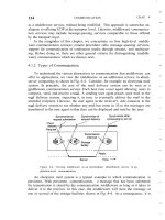
Figure 6.1: Signal and data flow in a digital communications system
(Couch, 1997)
Figure 6.2: Signal coding by frequently changing line codes in RFID

systems
Figure 6.3: Generating differential coding from NRZ coding
Figure 6.4: Possible signal path in pulse-pause coding
Figure 6.5: Each modulation of a sinusoidal signal — the carrier —
generates so-called (modulation) sidebands
Figure 6.6: In ASK modulation the amplitude of the carrier is switched
between two states by a binary code signal
Figure 6.7: The generation of 100% ASK modulation by the keying of
the sinusoidal carrier signal from a HF generator into an ASK
modulator using a binary code signal
Figure 6.8: Representation of the period duration T and the bit duration
τ of a binary code signal
Figure 6.9: The generation of 2 FSK modulation by switching between
two frequencies f
1
and f
2
in time with a binary code signal
Figure 6.10: The spectrum of a 2 FSK modulation is obtained by the
addition of the individual spectra of two amplitude shift keyed
oscillations of frequencies f
1
and f
2
Figure 6.11: Generation of the 2 PSK modulation by the inversion of a
sinusoidal carrier signal in time with a binary code signal
Figure 6.12: Step-by-step generation of a multiple modulation, by load
modulation with ASK modulated subcarrier
Figure 6.13: Modulation products using load modulation with a
subcarrier

Chapter 7: Data Integrity
This document was created by an unregistered ChmMagic, please go to to register it. Thanks.
Figure 7.1: Interference during transmission can lead to errors in the
data
Figure 7.2: The parity of a byte can be determined by performing
multiple exclusive-OR logic gating operations on the individual bits
Figure 7.3: If the LCR is appended to the transmitted data, then a new
LRC calculation incorporating all received data yields the checksum
00h. This permits a rapid verification of data integrity without the
necessity of knowing the actual LRC sum
Figure 7.4: Step-by-step calculation of a CRC checksum
Figure 7.5: If the CRC is appended to the transmitted data a repeated
CRC calculation of all received data yields the checksum 0000h. This
facilitates the rapid checking of data integrity without knowing the CRC
total
Figure 7.6: Operating principle for the generation of a CRC-16/CCITT
by shift registers
Figure 7.7: The circuit for the shift register configuration outlined in the
text for the calculation of a CRC 16/CCITTT
Figure 7.8: Broadcast mode— the data stream transmitted by a reader
is received simultaneously by all transponders in the reader's
interrogation zone
Figure 7.9: Multi-access to a reader— numerous transponders attempt
to transfer data to the reader simultaneously
Figure 7.10: Multi-access and anticollision procedures are classified on
the basis of four basic procedures
Figure 7.11: Adaptive SDMA with an electronically controlled directional
antenna. The directional beam is pointed at the various transponders
one after the other
Figure 7.12: In an FDMA procedure several frequency channels are

available for the data transfer from the transponders to the reader
Figure 7.13: Classification of time domain anticollision procedures
according to Hawkes (1997)
Figure 7.14: Definition of the offered load G and throughput S of an
ALOHA system— several transponders send their data packets at
random points in time. Now and then this causes data collisions, as a
result of which the (data) throughput S falls to zero for the data packets
that have collided
Figure 7.15: Comparison of the throughput curves of ALOHA and
S-ALOHA. In both procedures the throughput tends towards zero as
soon as the maximum has been exceeded
Figure 7.16: Throughput behaviour taking into account the capture
effect with thresholds of 3 dB and 10 dB
Figure 7.17: Transponder system with slotted ALOHA anticollision
procedure
This document was created by an unregistered ChmMagic, please go to to register it. Thanks.
Figure 7.18: Dynamic S-ALOHA procedure with BREAK command.
After the serial number of transponder 1 has been recognised without
errors, the response of any further transponders is suppressed by the
transmission of a BREAK command
Figure 7.19: Bit coding using Manchester and NRZ code
Figure 7.20: Collision behaviour for NRZ and Manchester code. The
Manchester code makes it possible to trace a collision to an individual
bit
Figure 7.21: The different serial numbers that are sent back from the
transponders to the reader in response to the REQUEST command
lead to a collision. By the selective restriction of the preselected
address range in further iterations, a situation can finally be reached in
which only a single transponder responds
Figure 7.22: Binary search tree. An individual transponder can finally

be selected by a successive reduction of the range
Figure 7.23: The average number of iterations needed to determine the
transponder address (serial number) of a single transponder as a
function of the number of transponders in the interrogation zone of the
reader. When there are 32 transponders in the interrogation zone an
average of six iterations are needed, for 65 transponders on average
seven iterations, for 128 transponders on average eight iterations, etc.
Figure 7.24: Reader's command (nth iteration) and transponder's
response when a 4-byte serial number has been determined. A large
part of the transmitted data in the command and response is redundant
(shown in grey). X is used to denote the highest value bit position at
which a bit collision occurred in the previous iteration
Figure 7.25: The dynamic binary search procedure avoids the
transmission of redundant parts of the serial number. The data
transmission time is thereby noticeably reduced
Chapter 8: Data Security
Figure 8.1: Mutual authentication procedure between transponder and
reader
Figure 8.2: In an authentication procedure based upon derived keys, a
key unique to the transponder is first calculated in the reader from the
serial number (ID number) of the transponder. This key must then be
used for authentication
Figure 8.3: Attempted attacks on a data transmission. Attacker 1
attempts to eavesdrop, whereas attacker 2 maliciously alters the data
Figure 8.4: By encrypting the data to be transmitted, this data can be
effectively protected from eavesdropping or modification
Figure 8.5: In the one-time pad, keys generated from random numbers
(dice) are used only once and then destroyed (wastepaper basket).
The problem here is the secure transmission of the key between
sender and recipient

This document was created by an unregistered ChmMagic, please go to to register it. Thanks.
Figure 8.6: The principle underlying the generation of a secure key by a
pseudorandom generator
Figure 8.7: Basic circuit of a pseudorandom generator incorporating a
linear feedback shift register (LFSR)
Chapter 9: Standardisation
Figure 9.1: Path of the activation field of a reader over time— no
transponder in interrogation zone, full/half duplex (= load
modulated) transponder in interrogation zone, sequential
transponder in the interrogation zone of the reader
Figure 9.2: Automatic synchronisation sequence between readers A
and B. Reader A inserts an extended pause of a maximum of 30 ms
after the first transmission pulse following activation so that it can listen
for other readers. In the diagram, the signal of reader B is detected
during this pause. The reactivation of the activation field of reader B
after the next 3 ms pause triggers the simultaneous start of the pulse
pause cycle of reader A
Figure 9.3: Structure of the load modulation data telegram comprising
of starting sequence (header), ID code, checksum and trailer
Figure 9.4: Signal path at the antenna of a reader
Figure 9.5: A sequential advanced transponder is switched into
advanced mode by the transmission of any desired command
Figure 9.6: Structure of an ISO 14223 command frame for the
transmission of data from reader to transponder
Figure 9.7: Structure of an ISO 14223 response frame for the
transmission of data from transponder to the reader
Figure 9.8: Family of (contactless and contact) smart cards, with the
applicable standards
Figure 9.9: Position of capacitive (E1–E4) and inductive coupling
elements (H1–H4) in a close coupling smart card

Figure 9.10: Half opened reader for close coupling smart cards in
accordance with ISO 10536. In the centre of the insertion slot four
capacitive coupling areas can be seen, surrounded by four inductive
coupling elements (coils) (reproduced by permission of Denso
Corporation, Japan — Aichi-ken)
Figure 9.11: Typical field strength curve of a reader for proximity
coupling smart cards (antenna current i
1
= 1A, antenna diameter D =
15 cm, number of windings N = 1)
Figure 9.12: Modulation procedure for proximity coupling smart cards in
accordance with ISO 14443 — Type A— Top— Downlink — ASK
100% with modified Miller coding (voltage path at the reader antenna).
Bottom— Uplink — load modulation with ASK modulated 847 kHz
subcarrier in Manchester coding (voltage path at the transponder coil)
This document was created by an unregistered ChmMagic, please go to to register it. Thanks.
Figure 9.13: The oscillogram of a signal generated at the reader
antenna by a Type A card using load modulation with an ASK
modulated subcarrier
Figure 9.14: Modulation procedure for proximity coupling smart cards in
accordance with ISO 14443 — Type B. Top— Downlink — ASK 10%
with NRZ coding (voltage path at the reader antenna). Bottom— Uplink
— load modulation with BPSK modulated 847 kHz subcarrier in NRZ
coding (voltage path at the transponder coil)
Figure 9.15: The oscillogram of a signal generated at the reader
antenna by a Type B card using load modulation with BPSK modulated
subcarrier
Figure 9.16: State diagram of a Type A smart card in accordance with
ISO 14443 (Berger, 1998)
Figure 9.17: The reader's Request command for Type A cards (REQA)

is made up of only 7 data bits. This reliably rules out the
misinterpretation of useful data destined for another card as a
REQUEST command (S = start of frame, E = end of frame)
Figure 9.18: With the exception of the REQA command and data
transmitted during the anticollision routine, all data sent between
reader and card (i.e. command, response and useful data) is
transferred in the form of standard frames. This always begins with a
start-of-frame signal (S), followed by any desired number of data bytes.
Each individual data byte is protected against transmission errors by a
parity bit. The data transmission is concluded by an end-of-frame
signal (E)
Figure 9.19: A dynamic binary search tree algorithm is used for the
determination of the serial number of a card. The serial numbers can
be 4, 7 or 10 bytes long, so the algorithm has to be run several times at
different cascade levels (CL)
Figure 9.20: State diagram of a Type B smart card in accordance with
ISO 14443
Figure 9.21: Structure of an REQB command. In order to reliably rule
out errors the anticollision prefix (Apf) possess a reserved value (05h),
which may not be used in the NAD parameter of a different command
Figure 9.22: Structure of an ATQB (Answer To Request B)
Figure 9.23: Structure of a slot marker. The sequential number of the
following slot is coded in the parameter APn— APn = 'nnnn 0101b' =
'n5h'; n = slot marker 1–15
Figure 9.24: Structure of a standard frame for the transmission of
application data in both directions between the reader and a Type B
card. The value x5h (05h, 15h, 25h, E5h, F5h) of the NAD (node
address) are subject to anticollision commands, in order to reliably rule
out confusion with application commands
Figure 9.25: A card is selected by the sending of an application

command preceded by the ATTRIB prefix, if the identifier of the card
corresponds with the identifier (PUPI) of the prefix
This document was created by an unregistered ChmMagic, please go to to register it. Thanks.
Figure 9.26: After anticollision the ATS of the card is requested
Figure 9.27: The ISO/OSI layer model in a smart card
Figure 9.28: Structure of the frame in ISO 14443. The data of the
application layer, Layer 7 (grey), are packed into the protocol frame of
the transport layer (white)
Figure 9.29: Coding of the PCB byte in a frame. The entire
transmission behaviour is controlled by the PCB (protocol control byte)
in the protocol
Figure 9.30: The '1 of 256' coding is generated by the combination of
512 time slots of 9.44 µs length. The value of the digit to be transferred
in the value range 0–255 can be determined from the position in time of
a modulation pulse. A modulation pulse can only occur at an uneven
time slot (1, 3, 5, 7, )
Figure 9.31: Structure of a message block (framing) made up of frame
start signal (SOF), data and frame end signal (EOF)
Figure 9.32: Coding of the SOF signal at the beginning of a data
transmission using '1 of 256' coding
Figure 9.33: The EOF signal consists of a modulation pulse at an even
time slot (t = 2) and thus is clearly differentiated from useful data
Figure 9.34: The SOF signal of '1 of 4' coding consists of two 9.44 µs
long modulation pulses separated by an interval of 18.88 µs
Figure 9.35: '1 of 4' coding arises from the combination of eight time
slots of 9.44 µs length. The value of the digit to be transmitted in the
value range 0–3 can be determined from the time position of a
modulation pulse
Figure 9.36: Measuring bridge circuit for measuring the load modulation
of a contactless smart card in accordance with ISO 14443

Figure 9.37: Mechanical structure of the measurement bridge,
consisting of the field generator coil (field coil), the two sensor coils
(sense and reference coil) and a smart card (PICC) as test object
(DUT) (reproduced by permission of Philips Semiconductors,
Hamburg)
Figure 9.38: Circuit of a reference card for testing the power supply of a
contactless smart card from the magnetic HF field of a reader
Figure 9.39: Format of a data carrier for tools and cutters
Figure 9.40: Coding of data bits using the modified FSK subcarrier
procedure
Figure 9.41: Electronic article surveillance system in practical operation
(reproduced by permission of METO EAS-System 2002, Esselte Meto,
Hirschborn)
Figure 9.42: Left, measuring points in a gateway for inspection using
artificial products; right, artificial product
Figure 9.43: Official logo of the GTAG initiative ()
This document was created by an unregistered ChmMagic, please go to to register it. Thanks.
Chapter 10: The Architecture of Electronic Data
Carriers
Figure 10.1: Overview of the different operating principles used in RFID
data carriers
Figure 10.2: Block diagram of an RFID data carrier with a memory
function
Figure 10.3: Block diagram of the HF interface of an inductively coupled
transponder with a load modulator
Figure 10.4: Generation of a load modulation with modulated
subcarrier— the subcarrier frequency is generated by a binary division
of the carrier frequency of the RFID system. The subcarrier signal itself
is initially ASK or FSK modulated (switch position ASK/FSK) by the
Manchester coded data stream, while the modulation resistor in the

transponder is finally switched on and off in time with the modulated
subcarrier signal
Figure 10.5: Example circuit of a HF interface in accordance with ISO
14443
Figure 10.6: A 100% ASK modulation can be simply demodulated by
an additional diode
Figure 10.7: Block diagram of address and security logic module
Figure 10.8: Block diagram of a state machine, consisting of the state
memory and a backcoupled switching network
Figure 10.9: Example of a simple state diagram to describe a state
machine
Figure 10.10: Block diagram of a read-only transponder. When the
transponder enters the interrogation zone of a reader a counter begins
to interrogate all addresses of the internal memory (PROM)
sequentially. The data output of the memory is connected to a load
modulator which is set to the baseband code of the binary code
(modulator). In this manner the entire content of the memory (128-bit
serial number) can be emitted cyclically as a serial data stream
(reproduced by permission of TEMIC Semiconductor GmbH,
Heilbronn)
Figure 10.11: Size comparison— low-cost transponder chip in the eye
of a needle (reproduced by permission of Philips Electronics N.V.)
Figure 10.12: Block diagram of a writable transponder with a
cryptological function to perform authentication between transponder
and reader (reproduced by permission of TEMIC Semiconductor
GmbH, Heilbronn)
Figure 10.13: A transponder with two key memories facilitates the
hierarchical allocation of access rights, in connection with the
authentication keys used
Figure 10.14: Several applications on one transponder — each

protected by its own secret key
This document was created by an unregistered ChmMagic, please go to to register it. Thanks.
Figure 10.15: Differentiation between fixed segmentation and free
segmentation
Figure 10.16: Example of a transponder with fixed segmentation of the
memory (IDESCO MICROLOG®) The four 'pages' can be protected
against unauthorised reading or writing using different passwords
(IDESCO, n.d.)
Figure 10.17: Memory configuration of a MIFARE® data carrier. The
entire memory is divided into 16 independent sectors. Thus a
maximum of separate 16 applications can be loaded onto a MIFARE®
card
Figure 10.18: The data structure of the MIFARE® application directory
consists of an arrangement of 15 pointers (ID1 to ID$F), which point to
the subsequent sectors
Figure 10.19: Data structure of the MIFARE® application directory— it
is possible to find out what applications are located in each sector from
the contents of the 15 pointers (ID1 to ID$F)
Figure 10.20: Block diagram of a dual port EEPROM. The memory can
be addressed either via the contactless HF interface or an IIC bus
interface (reproduced by permission of Atmel Corporation, San Jose,
USA)
Figure 10.21: Pin assignment of a dual port EEPROM. The
transponder coil is contacted to pins L
1
and L
2
. All other pins of the
module are reserved for connection to the I
2

C bus and for the power
supply in 'contact mode' (reproduced by permission of Atmel
Corporation, San Jose, USA)
Figure 10.22: Memory configuration of the AT24RF08. The available
memory of 1 Kbyte is split into 16 segments (blocks 0-7) of 128 bytes
each. An additional memory of 32 bytes contains the access protection
page and the unique serial numbers. The access protection page
permits different access rights to be set in the memory for the HF and
I
2
C bus interface
Figure 10.23: The access configuration matrix of the module
AT24RF08 facilitates the independent setting of access rights to the
blocks 0–7
Figure 10.24: Block diagram of a transponder with a microprocessor.
The microprocessor contains a coprocessor (cryptological unit) for the
rapid calculation of the cryptological algorithms required for
authentication or data encryption
Figure 10.25: Command processing sequence within a smart card
operating system (Rankl and Effing, 1996)
Figure 10.26: Possible layout of a dual interface smart card. The chip
module is connected to both contact surfaces (like a telephone smart
card) and a transponder coil (reproduced by permission of Amatech
GmbH & Co. KG, Pfronten)
Figure 10.27: Block diagram of a dual interface card. Both smart card
interfaces can be addressed independently of one another
This document was created by an unregistered ChmMagic, please go to to register it. Thanks.
Figure 10.28: Block diagram of the MIFARE®-plus 'dual interface card'
chip. In contactless operating mode the common EEPROM is
accessed via a MIFARE®-compatible state machine. When operating

via the contact interface a microprocessor with its own operating
system accesses the same memory (reproduced by permission of SLE
44R42, Infineon AG, Munich)
Figure 10.29: Block diagram of the dual interface card chip 'MIFARE
ProX' (reproduced by permission of Philips Semiconductors Gratkorn,
A-Gratkorn)
Figure 10.30: Calculation of the 3DES (triple DES). Encryption (above)
and decryption (below) of a data block (reproduced by permission of
Philips Semiconductors Gratkorn, A-Gratkorn)
Figure 10.31: Block diagram of a DES coprocessor. The CPU key and
data can be transferred to the coprocessor by means of its own SFR
(special function register) (reproduced by permission of Philips
Semiconductors Gratkorn, A-Gratkorn)
Figure 10.32: Simplified functional block diagram of a (S)RAM cell
Figure 10.33: The EEPROM cell consists of a modified field effect
transistor with an additional floating gate
Figure 10.34: Basic configuration of a ferroelectric crystal lattice— an
electric field steers the inner atom between two stable states
Figure 10.35: FRAM cell structure (1 bit) and hysteresis loop of the
ferroelectric capacitor
Figure 10.36: Inductively coupled transponder with additional
temperature sensor
Figure 10.37: Distance and speed measurements can be performed by
exploiting the Doppler effect and signal travelling times
Figure 10.38: Influence of quantities on the velocity v of the surface
wave in piezocrystal are shear, tension, compression and temperature.
Even chemical quantities can be detected if the surface of the crystal is
suitably coated (reproduced by permission of Technische Universitä
Wien, Institut für allgemeine Elektrotechnik und Elektronik)
Figure 10.39: Arrangement for measuring the temperature and torque

of a drive shaft using surface wave transponders. The antenna of the
transponder for the frequency range 2.45 GHz is visible on the picture
(reproduced by permission of Siemens AG, ZT KM, Munich)
Figure 10.40: A surface wave transponder is used as a pressure
sensor in the valve shaft of a car tyre valve for the wireless
measurement of tyre pressure in a moving vehicle (reproduced by
permission of Siemens AG, ZT KM, Munich
Chapter 11: Readers
Figure 11.1: Master-slave principle between application software
(application), reader and transponder
This document was created by an unregistered ChmMagic, please go to to register it. Thanks.
Figure 11.2: Block diagram of a reader consisting of control system and
HF interface. The entire system is controlled by an external application
via control commands
Figure 11.3: Example of a reader. The two functional blocks, HF
interface and control system, can be clearly differentiated (MIFARE®
reader, reproduced by permission of Philips Electronics N.V.)
Figure 11.4: Block diagram of an HF interface for an inductively
coupled RFID system
Figure 11.5: Block diagram of an HF interface for microwave systems
Figure 11.6: Layout and operating principle of a directional coupler for a
backscatter RFID system
Figure 11.7: HF interface for a sequential reader system
Figure 11.8: Block diagram of a reader for a surface wave transponder
Figure 11.9: Block diagram of the control unit of a reader. There is a
serial interface for communication with the higher application software
Figure 11.10: Signal coding and decoding is also performed by the
control unit in the reader
Figure 11.11: The low-cost reader IC U2270B represents a highly
integrated HF interface. The control unit is realised in an external

microprocessor (MCU) (reproduced by permission of TEMIC
Semiconductor GmbH, Heilbronn)
Figure 11.12: Block diagram of the reader IC U2270B. The transmitter
arm consists of an oscillator and driver to supply the antenna coil. The
receiver arm consists of filter, amplifier and a Schmitt trigger
(reproduced by permission of TEMIC Semiconductor GmbH,
Heilbronn)
Figure 11.13: Rectification of the amplitude modulated voltage at the
antenna coil of the reader (reproduced by permission of TEMIC
Semiconductor GmbH, Heilbronn)
Figure 11.14: Block diagram for the reader IC U2270B with connected
antenna coil at the push-pull output (reproduced by permission of
TEMIC Semiconductor GmbH, Heilbronn)
Figure 11.15: Driver circuit in the reader IC UU2270B (reproduced by
permission of TEMIC Semiconductor GmbH, Heilbronn)
Figure 11.16: Complete example application for the low cost reader IC
U2270B (reproduced by permission of TEMIC Semiconductor GmbH,
Heilbronn)
Figure 11.17: Connection of an antenna coil using 50 O technology
Figure 11.18: Simple matching circuit for an antenna coil
Figure 11.19: Reader with integral antenna and matching circuit
(MIFARE®-reader, reproduced by permission of Philips Electronics
N.V.)
This document was created by an unregistered ChmMagic, please go to to register it. Thanks.
Figure 11.20: Representation of Z
A
in the impedance level (Z plane)
Figure 11.21: Transformation path with C
ls
and C

2p
Figure 11.22: The matching circuit represented as a current divider
Figure 11.23: Example of an OEM reader for use in terminals or robots
(photo— Long-Range/High-Speed Reader LHRI, reproduced by
permission of SCEMTEC Transponder Technology GmbH,
Reichshof-Wehnrath)
Figure 11.24: Reader for portable use in payment transactions or for
service purposes. (Photo of LEGIC® reader reproduced by permission
of Kaba Security Locking Systems AG, CH-Wetzikon)
Chapter 12: The Manufacture of Transponders
and Contactless Smart Cards
Figure 12.1: Transponder manufacture
Figure 12.2: Size comparison of a sawn die with a cereal grain. The
size of a transponder chip varies between 1 mm
2
and 15 mm
2
depending upon its function (photo— HITAG® Multimode-Chip,
reproduced by permission of Philips Electronics N.V.)
Figure 12.3: Manufacture of plastic transponders. In the figure an
endless belt is fitted with transponder coils wound onto a ferrite core.
After the transponder chip has been fitted and contacted, the
transponder on the belt is sprayed with plastic (reproduced by
permission of AmaTech GmbH & Co. KG, Pfronten)
Figure 12.4: Foil structure of a contactless smart card
Figure 12.5: Production of a semi-finished transponder by winding and
placing the semifinished transponder on an inlet sheet (reproduced by
permission of AmaTech GmbH & Co. KG, Pfronten)
Figure 12.6: Manufacture of an inlet sheet using the embedding
principle (reproduced by permission of AmaTech GmbH & Co. KG,

Pfronten)
Figure 12.7: Manufacture of a smart card coil using the embedding
technique on an inlet foil. The sonotrodes, the welding electrodes (to
the left of the sonotrodes) for contacting the coils, and some finished
transponder coils are visible (reproduced by permission of AmaTech
GmbH & Co. KG, Pfronten)
Figure 12.8: Example of a 13.56 MHz smart card coil using screen
printing technology
Figure 12.9: Contacting of a chip module to a printed or etched antenna
by means of cut clamp technology
Figure 12.10: Soldered connection between the chip module and an
etched antenna
Figure 12.11: During the lamination procedure the PVC sheets are
melted at high pressure and temperatures up to 150 °C
This document was created by an unregistered ChmMagic, please go to to register it. Thanks.
Figure 12.12: After the cooling of the PVC sheets the individual cards
are stamped out of the multi-purpose sheets
Chapter 13: Example Applications
Figure 13.1: The large 'family' of smart cards, including the relevant
ISO standard
Figure 13.2: The main fields of application for contactless smart cards
are public transport and change systems for telephone boxes or
consumer goods (groceries, cigarettes) (reproduced by permission of
Philips Electronics N.V.)
Figure 13.3: Contactless reader in a public transport system (photo—
Frydek-Mistek project, Czechoslovakia, source— reproduced by
permission of EM Test)
Figure 13.4: Use of the different tariff systems in a journey by public
transport. The journey shown involves two changes between the
underground and bus network. The number of times the smart card is

read depends upon the fare system used
Figure 13.5: Use of a contactless smart card in Seoul. A contactless
terminal is shown in communication with a contactless smart card in
the centre of the picture (reproduced by permission of Intec)
Figure 13.6: Contactless smart card for paying for journeys in a
scheduled bus in Seoul (reproduced by permission of Klaus
Finkenzeller, Munich)
Figure 13.7: Reader for contactless smart cards at the entrance of a
scheduled bus in Seoul (reproduced by permission of Klaus
Finkenzeller, Munich)
Figure 13.8: System components of the Fahrsmart system. The vehicle
equipment consists of a reader for contactless smart cards, which is
linked to the on-board computer. Upon entry into the station, the record
data is transferred from the on-board computer to a depot server via an
infrared link
Figure 13.9: Fahrsmart II contactless smart card, partially cut away.
The transponder coil is clearly visible at the lower right-hand edge of
the picture (reproduced by permission of Giesecke & Devrient, Munich)
Figure 13.10: The contactless FlexPass of the district of Constance
showing the GeldKarte and envelope (reproduced by permission of
TCAC GmbH, Dresden)
Figure 13.11: Contactless transaction using the FlexPass at a reader
(reproduced by permission of TCAC GmbH, Dresden)
Figure 13.12: Miles & More — Senator ChipCard, partially cut away.
The transponder module and antenna are clearly visible at the
right-hand edge of the picture underneath the hologram (reproduced by
permission of Giesecke & Devrient, Munich)
Figure 13.13: Passenger checking in using the contactless Miles &
More Frequent Flyer Card (reproduced by permission of Lufthansa)
This document was created by an unregistered ChmMagic, please go to to register it. Thanks.

Figure 13.14: Contactless reader as access control and till device at a
ski lift (reproduced by permission of Legic Identsystems, CH-Wetzikon)
Figure 13.15: To achieve mutual decoupling the readers are switched
alternately in time-division multiplex operation
Figure 13.16: Access control and time keeping are combined in a
single terminal. The watch with an integral transponder performs the
function of a contactless data carrier (reproduced by permission of
Legic® -Installation, Kaba Security Locking Systems AG,
CH-Wetzikon)
Figure 13.17: Offline terminal integrated into a doorplate. The lock is
released by holding the authorized transponder in front of it. The door
can then be opened by operating the handle. The door terminal can be
operated for a year with four 1.5 V Mignon batteries and even has a
real time clock that allows it to check the period of validity of the
programmed data carrier. The terminals themselves are programmed
by an infrared data transmission using a portable infrared reader
(reproduced by permission of Häfele GmbH, D-Nagold)
Figure 13.18: The hotel safe with integral offline terminal can only be
opened by an authorised data carrier (reproduced by permission of
(hotel-save is shown by the picture) Häfele GmbH, D-Nagold)
Figure 13.19: Euro balise in practical operation (reproduced by
permission of Siemens Verke-hrstechnik, Braunschweig)
Figure 13.20: Fitting a read antenna for the Euro balise onto a tractive
unit (reproduced by permission of Siemens Verkehrstechnik,
Braunschweig)
Figure 13.21: Container identification mark, consisting of owner's code,
serial number and a test digit
Figure 13.22: Size comparison of different variants of electronic animal
identification transponders— collar transponder, rumen bolus, ear tags
with transponder, injectible transponder (reproduced by permission of

Dr Michael Klindtworth, Bayrische Landesanstalt für Landtechnik,
Freising)
Figure 13.23: The options for attaching the transponder to a cow
Figure 13.24: Cross-sections of various transponder designs for animal
identification (reproduced by permission of Dr Georg Wendl,
Landtechnischer Verein in Bayern e.V., Freising)
Figure 13.25: Enlargement of different types of glass transponder
(reproduced by permission of Texas Instruments)
Figure 13.26: Injection of a transponder under the scutulum of a cow
(reproduced by permission of Dr Georg Wendl, Landtechnischer Verein
in Bayern e.V., Freising)
Figure 13.27: Automatic identification and calculation of milk production
in the milking booth (reproduced by permission of Dr Georg Wendl,
Landtechnischer Verein in Bayern e.V., Freising)
Figure 13.28: Output related dosing of concentrated feed at an
This document was created by an unregistered ChmMagic, please go to to register it. Thanks.