COMPUTER-AIDED INTELLIGENT RECOGNITION TECHNIQUES AND APPLICATIONS phần 8 pdf

References 343
[22] McLaughlin, R. A. and Alder, M. D. The Hough Transform versus the UpWrite, TR97-02, CIIPS,
The University of Western Australia, 1997.
[23] Milisavljevi
´
c, N. “Comparison of Three Methods for Shape Recognition in the Case of Mine Detection,”
Pattern Recognition Letters, 20(11–13), pp. 1079–1083, 1999.
[24] Haig, T., Attikiouzel, Y. and Alder, M. D. “Border Following: New Definition Gives Improved Border,” IEE
Proceedings-I, 139(2), pp. 206–211, 1992.
[25] McLaughlin, R. A. Randomized Hough Transform: Improved Ellipse Detection with Comparison, TR97-01,
CIIPS, The University of Western Australia, 1997.
[26] Xu, L. “Randomized Hough Transform (RHT): Basic Mechanisms, Algorithms and Computational
Complexities,” CVGIP: Image Understanding, 57(2), pp. 131–154, 1993.
[27] Xu, L., Oja, E. and Kultanen, P. “A New Curve Detection Method: Randomized Hough Transform (RHT),”
Pattern Recognition Letters, 11, pp. 331–338, 1990.
[28] Duda, O. and Hart, P. E. “Use of the Hough Transform to Detect Lines and Curves in Pictures,”
Communications of the Association for Computing Machinery, 15(1), pp. 11–15, 1972.
[29] Kälviäinen, H., Hirvonen, P., Xu, L. and Oja, E. “Comparisons of Probabilistic and Non-Probabilistic Hough
Transforms,” Proceedings of 3rd European Conference on Computer Vision, Stockholm, Sweden, pp. 351–360,
1994.
[30] Leavers, V. F. Shape Detection in Computer Vision Using the Hough Transform, Springer, London, 1992.
[31] Yuen, H. K., Illingworth, J. and Kittler, J. “Detecting Partially Occluded Ellipses using the Hough Transform,”
Image and Vision Computing, 7(1), pp. 31–37, 1989.
[32] Capineri, L., Grande, P. and Temple, J. A. G. “Advanced Image-Processing Technique for Real-Time
Interpretation of Ground Penetrating Radar Images,” International Journal on Imaging Systems and
Technology, 9, pp. 51–59, 1998.
[33] Milisavljevi
´
c, N., Bloch, I. and Acheroy, M. “Application of the Randomized Hough Transform to
Humanitarian Mine Detection,” Proceedings of the 7th IASTED International Conference on Signal and Image
Procesing (SIP2001), Honolulu, Hawaii, USA, pp. 149–154, 2001.

[34] Banks, E. Antipersonnel Landmines – Recognising and Disarming, Brassey’s, London-Washington, 1997.
[35] Milisavljevi
´
c, N. and Bloch, I. “Sensor Fusion in Anti-Personnel Mine Detection Using a Two-Level Belief
Function Model,” IEEE Transactions On Systems, Man, and Cybernetics C, 33(2), pp. 269–283, 2003.
[36] Milisavljevi
´
c, N., Bloch, I., van den Broek, S. P. and Acheroy, M. “Improving Mine Recognition
through Processing and Dempster–Shafer Fusion of Ground-Penetrating Data,” Pattern Recognition, 36(5),
pp. 1233–1250, 2003.
[37] Dubois, D., Grabisch, M., Prade, H. and Smets, P. “Assessing the Value of a Candidate,” Proceedings of
15th Conference on Uncertainty in Artificial Intelligence (UAI’99), Stockholm, Sweden, pp. 170–177, 1999.
[38] Smets, P. “Belief Functions: the Disjunctive Rule of Combination and the Generalized Bayesian Theorem,”
International Journal of Approximate Reasoning, 9, pp. 1–35, 1993.
[39] Schubert, J. “On Nonspecific Evidence,” International Journal of Intelligent Systems, 8, pp. 711–725, 1993.
[40] Smets, P. “Constructing the Pignistic Probability Function in a Context of Uncertainty,” Uncertainty in
Artificial Intelligence, 5, pp. 29–39, 1990.
[41] Milisavljevi
´
c, N., Bloch, I. and Acheroy, M. “Characterization of Mine Detection Sensors in Terms of Belief
Functions and their Fusion, First Results,” Proceedings of 3rd International Conference on Information Fusion
(FUSION 2000), II, pp. ThC3.15–ThC3.22, 2000.

18
Fast Object Recognition Using
Dynamic Programming from
a Combination of Salient Line
Groups
Dong Joong Kang
Jong Eun Ha

School of Information Technology, Tongmyong University of Information Technology,
Busan 608-711, Korea
In So Kweon
Department of Electrical & Computer Science Engineering, Korea Advanced Institute of
Science and Technology, Daejun, Korea
This chapter presents a new method of grouping and matching line segments to recognize objects.
Weproposeadynamicprogramming-basedformulationextractingsalientlinepatternsbydefiningarobust
and stable geometric representation that is based on perceptual organizations. As the end point proximity,
we detect several junctions from image lines. We then search for junction groups by using the collinear
constraint between the junctions. Junction groups similar to the model are searched in the scene, based on
a local comparison. A DP-based search algorithm reduces the time complexity for the search of the model
lines in the scene. The system is able to find reasonable line groups in a short time.
1. Introduction
This chapter describes an algorithm that robustly locates collections of salient line segments in an image.
In computer vision and related applications, we often wish to find objects based on stored models from
an image containing objects of interest [1–6]. To achieve this, a model-based object recognition system
Computer-Aided Intelligent Recognition Techniques and Applications Edited by M. Sarfraz
© 2005 John Wiley & Sons, Ltd
346 Fast Object Recognition Using DP
first extracts sets of features from the scene and the model, and then it looks for matches between
members of the respective sets. The hypothesized matches are then verified and possibly extended to be
useful in various applications. Verification can be accomplished by hypothesizing enough matches to
constrain the geometrical transformation from a 3D model to a 2D image under perspective projection.
We first extract junctions formed by two lines in the input image, and then find an optimal relation
between the extracted junctions, by comparing them with previously constructed model relations.
The relation between the junctions is described by a collinear constraint and parallelism can also be
imposed. Junction detection acts as a line filter to extract salient line groups in the input image and
then the relations between the extracted groups are searched to form a more complex group in an
energy minimization framework. The method is successfully applied to images with some deformation
and broken lines. Because the system can define a topological relation that is invariant to viewpoint

variations, it is possible to extract enough lines to guide 2D or 3D object recognition.
Conventionally, the DP-based algorithm as a search tool is an optimization technique for the problems
where not all variables are interrelated simultaneously [7–9]. In the case of an inhomogeneous problem,
such as object recognition, related contextual dependency for all the model features always exists [10].
Therefore, DP optimization would not give the true minimum.
On the other hand, the DP method has an advantage in greatly reducing the time complexity for a
candidate search, based on the local similarity. Silhouette or boundary matching problems that satisfy
the locality constraint can be solved by DP-based methods using local comparison of the shapes. In
these approaches, both the model and matched scene have a sequentially connected form of lines,
ordered pixels, or chained points [11–13]. In some cases, there also exist many vision problems,
in which the ordering or local neighborhood cannot be easily defined. For example, definition of a
meaningful line connection in noisy lines is not easy, because the object boundary extraction for an
outdoor scene is itself a formidable job for object segmentation.
In this chapter, we do not assume known boundary lines or junctions, rather, we are open to any
connection possibilities for arbitrary junction groups in the DP-based search. That is, the given problem
is a local comparison between predefined and sequentially linked model junctions and all possible
scene lines in an energy minimization framework.
Section 2 introduces previous research about feature grouping in object recognition. Section 3
explains a quality measure to detect two line junctions in an input image. Section 4 describes a
combination model to form local line groups and how junctions are linked to each other. Section 5
explains how related junctions are searched to form the salient line groups in a DP-based search
framework. Section 6 gives a criterion to test the collinearity between lines. Section 7 tests the
robustness of the junction detection algorithm by counting the number of detected junctions as a
function of the junction quality and whether a prominent junction from a single object is extracted
under an experimentally decided quality threshold. Section 8 presents the results of experiments using
synthetic and real images. Finally, Section 9 summarizes the results and draws conclusions.
2. Previous Research
Guiding object recognition by matching perceptual groups of features was suggested by Lowe [6]. In
SCERPO, his approach is to match a few significant groupings from certain arrangements of lines
found in images. Lowe has successfully incorporated grouping into an object recognition system. First,

he groups together lines thought particularly likely to come from the same object. Then, SCERPO looks
for groups of lines that have some property invariant with the camera viewpoint. For this purpose, he
proposes three major line groups – proximity, parallelism and collinearity.
Recent results in the field of object recognition, including those of Jacobs, Grimson and Huttenlocher,
demonstrate the necessity of some type of grouping, or feature selection, to make the combinatorics of
object recognition manageable [9,14]. Grouping, as for the nonaccidental image features, overcomes
the unfavorable combinatorics of recognition by removing the need to search the space for all matches
Junction Extraction 347
between image and model features. Grimson has shown that the combinatorics of the recognition
process in cluttered environments using a constrained search reduces the time complexity from an
exponential to a low-order polynomial if we use an intermediate grouping process [9]. Only those
image features considered likely to come from a single object could be included together in hypothetical
matches. And these groups need only be matched with compatible groups of model features. For
example, in the case of a constrained tree search, grouping may tell us which parts of the search tree
to explore first, or allow us to prune sections of the tree in advance.
This chapter is related to Lowe’s work using perceptual groupings. However, the SCERPO grouping
has a limitation: forming only small groups of lines limits the amount by which we may reduce the
search. Our work extends the small grouping to bigger perceptual groups, including more complex
shapes. Among Lowe’s organization groups, the proximity consisting of two or more image lines is
an important clue for starting object recognition. When projected to the image plane, most manmade
objects may have a polyhedral plane in which two or several sides give line junctions. First, we
introduce a quality measure to detect meaningful line junctions denoting the proximity. The quality
measure must be carefully defined not to skip salient junctions in the input image. Then, extracted
salient junctions are combined to form more complex and important local line groups. The combination
between junctions is guided by the collinearity that is another of Lowe’s perceptual groups. Henikoff
and Shapiro [15] effectively use an ordered set of three lines representing a line segment with junctions
at both ends. In their work, the line triples, or their relations as a local representative pattern, broadly
perform the object recognition and shape indexing. However, their system cannot define the line triple
when the common line sharing two junctions is broken by image noise or object occlusion. And the
triple and bigger local groups are separately defined in low-level detection and discrete relaxation,

respectively. The proposed system in this chapter is able to form the line triple and bigger line groups
in a consistent framework. Although the common line is broken, the combination of the two junctions
can be compensated by the collinearity of the broken lines. We introduce the following:
1. A robust and stable geometric representation that is based on the perceptual organizations (i.e. the
representation as a primitive search node includes two or more perceptual grouping elements).
2. A consistent search framework combining the primitive geometric representations, based on the
dynamic programming formulation.
3. Junction Extraction
A junction is defined as any pair of line segments that intersect, and whose intersection point either lies
on one of the line segments, or does not lie on either of the line segments. An additional requirement is
that the acute angle between the two lines must lie in a range 
min
to 
max
. In order to avoid ambiguity
with parallel or collinear pairs [6], 
min
could be chosen to be a predefined threshold. Various junction
types are well defined by Etemadi et al. [7].
Now a perfect junction (or two-line junction) is defined as one in which the intersection point P
lies precisely at the end points of the line segments. Figure 18.1 shows the schematic diagram of a
typical junction. Note that there are now two virtual lines that share the end point P. The points P
1
and P
4
locating the opposite sides of P
2
and P
3
, denote the remaining end points of the virtual lines,

respectively. Then, the junction quality factor is:
Q
J
=
L
1
−

1
−
⊥
2
VL
1

·
L
2
−

2
−
⊥
1
VL
2

(18.1)
where VL
i

i = 1 2 are the lengths of the virtual lines, as shown in Figure 18.1. The standard
deviations 

i
and 
⊥
i
, incorporating the uncertainties in the line extraction process for the
position of the end points of the line segments along and perpendicular to its direction respectively,
may be replaced by constants without affecting the basic grouping algorithms [7]. In this chapter, the
348 Fast Object Recognition Using DP
P
1
P
2
L
1
VL
1
P
4
L
2
P
3
VL
2
P
θ
Figure 18.1 The junction.

two variance factors 

i
and 
⊥
i
are ignored. The defined relation penalizes pairings in which either
line is far away from the junction point. The quality factor also retains the symmetry property.
4. Energy Model for the Junction Groups
The relational representation, made from each contextual relation of the model and scene features,
provides a reliable means to compute the correspondence information in the matching problem. Suppose
that the model consists of M feature nodes. Then, a linked node chain, given by the sequential
connection of the nodes, can be constructed.
If the selected features are sequentially linked, then it is possible to calculate a potential energy from
the enumerated feature nodes. For example, assume that any two-line features of the model correspond
to two features f
I
and f
I+1
of the scene. If the relational configuration of each line node depends only
on the connected neighboring nodes, then the energy potential obtained from the M line nodes can be
represented as:
E
total
f
1
f
2
f
M

 = E
1
f
1
f
2
 +E
2
f
2
f
3
 +···+E
M−1
f
M−1
f
M
 (18.2)
where
E
I
f
I
f
I+1
 =
K

k =1

r
2k
f
I
f
I+1
 −R
2k
I I +1 (18.3)
Here, r
2k
and R
2k
denote the binary relations of any two connected line features of the scene and the
model, respectively. The parameter K is the number of binary relations.
For the relational representation of junctions, the model and scene node I and f
I
in Equations (18.2)
and (18.3) are replaced by the model junction and corresponding scene junction, respectively.
Figure 18.2(a) presents a schematic of lines consisting of an object. Figure 18.2(b) shows the binary
relations of sequentially connected junctions for line pattern matching. Equation (18.3) for junction
chains can be rewritten accordingly as:
E
I
f
I
f
I+1
 =  ·f
I

 −I+ ·rf
I
f
I+1
 −RI I +1 (18.4)
Each junction has the unary angle relation from two lines constituting a single junction, as shown in
the first term of Equation (18.4) and in Figure 18.1. f
I
 and I are corresponding junction angles
in a scene and a model, respectively. We do not use a relation depending on line length, because lines
in a noisy scene could be easily broken. The binary relation for the scene r and model R in the
Energy Minimization 349
1
2
3
4
6
(a)
J
1
J
2
1
2
3
4
5
6
++ + . . .
J

3
(b)
5
Figure 18.2 Binary relations made from any two connected junction nodes: (a) line segments on a
model; and (b) the combination of junctions by perceptual constraints, such as proximity, collinearity
and parallelism.
second term is defined as a topological constraint or an angle relation between two junctions. For
example, the following descriptions can represent the binary relations.
1. Two lines 1 and 4 should be approximately parallel (parallelism).
2. Scene lines corresponding to two lines 2 and 3 must be a collinear pair [6] or the same line. That
is, two junctions are combined by the collinear constraint.
3. Line ordering for two junctions J
1
, J
2
should be maintained, for example as clockwise or counter-
clockwise, as the order of line 1, line 2, line 3 and line 4.
The relation defined by the connected two junctions includes all three perceptual organization groups
that Lowe used in SCERPO. These local relations can be selectively imposed according to the type
of the given problem. For example, a convex line triplet [15] is simply defined, by removing the
above constraint 1 and letting line 2 and line 3 of constraint 2 be equal to each other. The weighting
coefficients  and  of the energy potential are experimentally given, by considering the variance
factor of the line perturbation for image noise.
5. Energy Minimization
Dynamic Programming (DP) is an optimization technique good for problems where not all variables
are interrelated simultaneously [8,16]. Suppose that the global energy can be decomposed into the
following form:
Ef
1
f

M
 = E
1
f
1
f
2
 +E
2
f
2
f
3
 +···+E
M−1
f
M−1
f
M
 (18.5)
in which M is the number of the model nodes, such as lines or junctions, and f
I
is a scene label that
can be assigned to the model node I.
Figure 18.3 shows a schematic DP diagram to find a trapezoidal model in the scene lines.
Figure 18.3(a) presents a typical case in which we cannot define an ordering for the scene lines due
350 Fast Object Recognition Using DP
(a)
(b)
1

2
.
. .
. . .
m + 1
Junction list
NIL NIL NIL
12 M
Figure 18.3 The DP algorithm searches a scene node corresponding to each model node. A model
feature can be matched to at least one node, among scene nodes, 1m+1 of a column, including
NULL node (NIL). (a) Line segments for the rear view of a vehicle; and (b) a DP-based search. m is
the number of junctions detected from (a) and M is the number of predefined model junctions.
to the cluttered background. Therefore, it is difficult to extract a meaningful object boundary that
corresponds to the given model. In this case, the DP-based search structure is formulated as the column
in Figure 18.3(b), in which all detected scene features are simultaneously included in each column.
Each junction of the model can get a corresponding junction in the scene as well as a null node, which
indicates no correspondence. The potential matches are defined as the energy accumulation form of
Equation (18.5). From binary relations of junctions (i.e. arrows in Figure 18.3(b)) defined between
two neighboring columns, the local comparison-based method using the recursive energy accumulation
table of Equation (18.5) can give a fast matching solution.
The DP algorithm generates a sequence that can be written in the recursive form. For
I = 1M−1,
D
I
f
I+1
 = min
f
I
D

I−1
f
I
 +E
I
f
I
f
I+1
 (18.6)
with D
0
f
1
 = 0. The minimal energy solution is obtained by
min
f
Ef
1
f
M
 = min
f
M
D
M−1
f
M
 (18.7)
If each f

I
takes on m discrete values, then to compute D
I−1
f
I
 for each f
I
value, one must evaluate
the summation D
I−1
f
I−1
 +E
I−1
f
I−1
f
I
 for the m different f
I−1
values. Therefore, the overall
minimization involves M −1m
2
evaluations of the summations. This is a large reduction from the
exhaustive search for the total evaluation of Ef
1
f
M
. m is the number of junctions satisfying a
threshold for the junction quality in the scene.

Collinear Criterion of Lines 351
6. Collinear Criterion of Lines
Extraction of the image features such as points or lines is influenced by the conditions during image
acquisition. Because the image noise distorts the object shape in the images, we need to handle the
effect of the position perturbation in the features, and to decide a threshold or criterion to discard and
reduce the excessive noise. In this section, the noise model and the error propagation for the collinearity
test between lines are proposed. The Gaussian noise distribution for two end points of a line is an
effective and general approach, as referred to in Haralick [17] and Roh [18], etc. In this section, we use
the Gaussian noise model to compute error propagation for two-line collinearity and obtain a threshold
value resulting from the error variance test to decide whether the two lines are collinear or not.
The line collinearity can be decomposed into two terms of parallelism and normal distance defined
between the two lines being evaluated.
6.1 Parallelism
The parallelism is a function of eight variables:
p = cos
−1

a ·b

a

b


 where a =x
2
−x
1
and b = x
4

−x
3
(18.8)
or p =px
1
 x
2
 x
3
 x
4
 where x
i
= x
i
y
i
 1
T
(18.9)
The x
i
i = 14 denote image coordinates for four end points of the two lines and

a

presents
the length of vector a. To avoid the treatment of a trigonometric function in calculating the partial
derivatives of function p with respect to the image coordinates, we use a simpler function:
p


= cosp =
a ·b

a

b

= p

x
1
 x
2
 x
3
 x
4
 (18.10)
Let x
i
y
i
 be the true value and ˜x
i
 ˜y
i
 be the noisy observation of x
i
y

i
, then we have
˜x
i
= x
i
+
i
(18.11a)
˜y
i
= y
i
+
i
(18.11b)
where the noise terms 
i
and 
i
denote independently distributed noise terms having mean 0 and
variance 
2
i
. Hence:
E


i


= E


i

= 0 (18.12)
V


i

= V


i

= 
2
i
(18.13)
E


i

j

=



2
0
if i = j
0 otherwise
E


i

j

=


2
0
if i = j
0 otherwise
(18.14a)
E


i

j

= 0 (18.14b)
From these noisy measurements, we define the noisy parallel function,
˜p


˜x
1
 ˜y
1
 ˜x
2
 ˜y
2
 ˜x
3
 ˜y
3
 ˜x
4
 ˜y
4
 (18.15)
352 Fast Object Recognition Using DP
To determine the expected value and variance of ˜p

, we expand ˜p

as a Taylor series at
x
1
y
1
x
2
y

2
x
3
y
3
x
4
y
4
:
˜p

≈ p

+
4

i=1

˜x
i
−x
i

 ˜p

˜x
i
+˜y
i

−y
i

 ˜p

˜y
i

= p

+
4

i=1


i
 ˜p

˜x
i
+
i
 ˜p

˜y
i

(18.16)
Then, the variance of the parallel function becomes:

Varp

 = E

˜p

−p


2

= 
2
0
4

i=1


 ˜p

˜x
i

2
+

 ˜p

˜y

i

2

(18.17)
Hence, for a given two lines, we can determine a threshold:
p = 3 ·

E˜p

−p


2
 (18.18)
Because the optimal p

equals 1, any parallel two lines have to satisfy the following condition:
1−˜p

≤ p (18.19)
6.2 Normal Distance
A normal distance between any two lines is selected from among two distances d
1
and d
2
:
d
norm
= maxd

1
d
2
 (18.20)
where
d
1
=

a
1
x

m
+b
1
y

m
+c
1


a
2
1
+b
2
1


1
2
(18.21a)
d
2
=

a
2
x
m
+b
2
y
m
+c
2


a
2
2
+b
2
2

1
2
(18.21b)
The a

i
b
i
and c
i
are line coefficients for the i-line and x
m
y
m
 denotes the center point coordinate
of the first line, and x

m
y

m
 denotes the center of the second line. Similarly to the parallel case of
Section 6.1, the normal distance is also a function of eight variables:
d
norm
= dx
1
 x
2
 x
3
 x
4
 (18.22)
Through all processes similar to the noise model of Section 6.1, we obtain:

Varp

 = E

˜p

−p


2

= 
2
0
4

i=1


 ˜p

˜x
i

2
+

 ˜p

˜y

i

2

(18.23)
For the given two lines, we can also determine a threshold for the normal distance:
d = 3 ·

E
˜
d −d
2
 (18.24)
Because the optimal d equals 0, the normal distance for any two collinear lines has to satisfy the
following condition:
˜
d ≤ d (18.25)
Energy Model for the Junction Groups 353
7. Energy Model for the Junction Groups
In this section, we test the robustness of the junction detection algorithm by counting the number of
detected junctions as a function of the junction quality Q
J
of Equation (18.1). Figure 18.4 shows some
images of 2D and 3D objects under well-controlled lighting conditions and a cluttered outdoor scene.
We use Lee’s method [19] to extract lines.
Most junctions (i.e. more than 80 %) extracted from possible combinations of the line segments
are concentrated in the range 00∼10 of the quality measure, as shown in Figure 18.5. The three
experimental sets of Figure 18.4 give similar tendencies except for a small fluctuation at the quality
measure 0.9, as shown in Figure 18.5. At the quality level 0.5, the occupied portion of the junctions
relative to the whole range drops to less than 1 %.

When robust line features are extracted, Q
J
, as a threshold for the junction detection, does not
severely influence the number of extracted junctions. In good conditions, the extracted lines are
clearly defined along the object boundary and few cluttered lines exist in the scene, as shown in
Figure 18.4(a). Therefore, the extracted junctions are accordingly defined and give junctions with a
high junction quality factor, as shown in Figure 18.4(a). The parts plot in Figure 18.5 graphically
shows the high-quality junctions as the peak concentrated in the neighbor range of quality measure 0.9.
For Q
J
= 07, the detection ratio 1.24 (i.e. number of junctions/number of primitive lines) of
Figure 18.4(a) is decreased to 0.41 for the outdoor scene of Figure 18.4(c), indicating the increased effect
of the threshold (see also Table 18.1). The effect of threshold level for the number of junctions resulting
from distorted and broken lines is more sensitive to the outdoor scenes. That is, junction detection
(a) (b) (c)
Figure 18.4 Junction extraction: the number of junctions depends on the condition of the images.
Each column consists of an original image, line segments and junctions and their intersecting points
for quality measure 0.5, respectively. The small circles in the figure represent the intersection points
of two-line junctions. (a) Parts: a 2D scene under controlled lighting conditions; (b) blocks: an indoor
image with good lighting; and (c) cars: a cluttered image under an uncontrolled outdoor road scene.
354 Fast Object Recognition Using DP
0
1
2
3
4
5
135678910
Quality measure (×
0.1)

# of Junctions (%)
42
Parts Blocks Cars
Figure 18.5 The occupying percentage of junctions according to changes of the quality measure.
Table 18.1 Junction number vs. quality measure.
Q
J
= 03 Q
J
= 05 Q
J
= 07
# of lines L
n
 # of junctions (V
n
)
V
n
L
n
V
n
V
n
L
n
V
n
V

n
L
n
Parts 100 376 378 196 196 124 124
Blocks 130 543 411 196 151 90 07
Cars 137 466 34 180 131 56 041
under uncontrolled lighting conditions has a higher dependence on the change of junction quality as a
detection threshold.
With some additional experiments, we identify that the number of junctions in scenes does not vary
much, in spite of a low Q
J
. Usually, a junction quality of 0.5 is sufficient to give an adequate number
of junctions for most test scenes while not skipping the salient junctions, and without increasing the
time complexity of the DP-based search.
8. Experiments
We applied the proposed method to find a group of optimal line junctions. Test scenes included some
lines distorted by a variation of viewpoint. First, input images were processed to detect only the
strongest step edges. Edges were further filtered by discarding shorter edge segments. Junctions were
then inferred between the remaining line segments. When junctions were extracted from the lines, then
relative relations between the junctions were searched by using the criterion of Section 4, with the
collinear constraint that links two junctions.
To reduce the repeated computation for relations between line segments, all possible relations such
as inter-angles, collinear properties and junction qualities between lines were previously computed.
Experiments 355
8.1 Line Group Extraction
As an example of 2D line matching for a viewpoint variation, the rear-view of a vehicle was used.
The description of the model lines was given as a trapezoidal object. The model pattern could have
a clockwise combination of the constituting lines. Figure 18.6(a-1) shows the first and the last image
among a sequence of 30 images to be tested. With the cluttered background lines, a meaningful
boundary extraction of the object of interest was difficult, as shown in Figure 18.6(a-2). Figure 18.6

(a-3) shows the extraction of junctions in the two frames. A threshold for the quality measure Q
J
was
set at 0.5. Figure 18.6(a-4) shows optimal matching lines having the smallest accumulation energy
of Equation (18.7). In spite of some variations from the model shape, a reasonable matching result
was obtained. Unary and binary properties of Equation (18.4) were both used. Figure 18.6(b) shows
a few optimal matching results. In Figure 18.6(b), the model shape is well matched as the minimum
DP energy of Equation (18.7), in spite of the distorted shapes in the scenes. Matching was successful
for 25 frames out of 30 – a success ratio of 83 %. Failing cases result from line extraction errors in
low-level processing, in which lines could not be defined on the rear windows of vehicles.
(a-1)
(a-3) (a-4)
(a-2)
(b)
Figure 18.6 Object matching under weak perspective projection: a rear-window of a vehicle on the
highway was used. (a-1) The first and last images to be tested; (a-2) line extraction; (a-3) junction
detection for Q
J
= 05; (a-4) optimal model matching; (b) a few optimal matching results between the
first and last images.
356 Fast Object Recognition Using DP
(a)
(b)
Figure 18.7 Object matching in a synthetic image with broken and noisy lines.
Figure 18.7 shows experimental results for extracting a 2D polyhedral object. Figure 18.7(a) shows
a model as a pentagon shape with noisy and broken lines in the background region. All lines except
for the pentagon were randomly generated. Figure 18.7(b) shows a few matching results with small
DP energy. A total of six candidates were extracted as the matched results for generating hypotheses
for the object recognition. Each one is similar to the pentagon model shape. It is interesting to see the
last result because we did not expect this extraction.

Two topological combinations of line junctions are shown as model shapes in Figure 18.8. J
1
and
J
2
junctions are combined with a collinear constraint that also denotes the same rotating condition as
the clockwise direction in the case of Figure 18.8(a). The three binary relations in Section 4 all appear
in the topology of Figure 18.8. In the combination of J
2
and J
3
, the rotating direction between the
two junctions is reversed. In Figure 18.8(b), similar topology to Figure 18.8(a) is given, except for
the difference of rotating direction of the constituting junctions. Figure 18.9 presents an example of
extracting topological line groups to guide 3D object recognition. The topological shapes are invariant
to wide changes of view. That is, if there is no self-occlusion on the object, the interesting line groups
are possible to extract. Figure 18.9(a) shows the original image to be tested. After discarding the
shorter lines, Figure 18.9(b) presents the extracted lines with the numbering indicating the line index,
and Figure 18.9(c) and 18.9(d) give the matched line groups corresponding to the model shape of
Experiments 357
J
1
J
2
J
3
J
4
J
1

J
2
J
3
J
4
(a) (b)
Figure 18.8 Topological shapes for model description. (a) A model with clockwise rotation of the
starting junction; (b) a model with counter-clockwise direction for the starting junction.
Figure 18.8(a) and 18.8(b), respectively. In each extraction, there are enough line groups to guide a
hypothesis for 3D object recognition.
Table 18.2 presents the matching results in Figure 18.9 corresponding to the models of Figure 18.8.
All extractions are enumerated for each model.
The above experimental results demonstrate that the proposed framework can find similar shapes
even from a cluttered and distorted line set. By the local comparison-based matching criterion permitting
a shape distortion for the reference model shape, reasonable line grouping and shape matching are
possible, without increasing the time complexity. The grouping and the junction detection are all
performed in 1 s, on a Pentium II-600 desktop machine. In all test sets, any length ratio of the model
or scene lines has not been used, because the scene lines are easily broken in outdoor images. Angle
relations and line ordering between two neighboring junctions are well preserved, even in broken and
distorted line sets.
Figure 18.9 A topological shape extraction for 3D object recognition. (a) Original image; (b) line
extraction; and (c), (d) found topological shapes.
358 Fast Object Recognition Using DP
39
41
70
69
79
39

41
70
69
39
86
41
70
69
56
38
80
41
116
56
38
80
116
41
38
80
41
118
56
86
80
(c)
(d)
Figure 18.9 (continued)
Experiments 359
Table 18.2 The topological matching results.

J
1
J
2
J
3
J
4
Model 1 (39, 80) (80, 41) (41, 70) (70, 69)
(39, 79) (86, 41) (41, 70) (70, 69)
(39, 86) (86, 41) (41, 70) (70, 69)
Model 2 (118, 41) (41, 80) (80, 38) (38, 56)
(40, 41) (41, 80) (80, 38) (38, 56)
(106, 41) (41, 80) (80, 38) (38, 56)
(94, 41) (41, 80) (80, 38) (38, 56)
(116, 41) (41, 80) (80, 38) (38, 56)
8.2 Collinearity Tests for Random Lines
We tested the stability of the two collinear functions proposed in Section 6 by changing the standard
deviation as a threshold for four end points of the two constituting lines. The noise was modeled as
Gaussian random noise having mean 0 and variance 
2
0
.
A total of 70 lines were randomly generated in a rectangular region of size 100×100 in Figure 18.10,
hence the number of possible line pairs was
70
C
2
= 2415. Finally, only two line pairs were selected as
satisfying the two collinear conditions of Equation (18.19) and Equation (18.25) under 

0
=01. When
we reduced the variation value, there were a few collinear sets. By a simple definition of collinear
functions and control of the variance 
0
as Gaussian perturbation, we could systematically obtain the
collinear line set without referring to heuristic parameters.
100
90
80
70
60
50
40
30
20
10
0
0 10 20 30 40 50 60 70 80 90 100
(a)
x
y
Figure 18.10 Collinear lines according to the change of standard deviation 
0
as a threshold. (a) The
randomly generated original line set; (b) line pairs detected for 
0
= 04; (c) for 
0
= 03; and (d) for


0
= 01.
360 Fast Object Recognition Using DP
(c) (d)(b)
Figure 18.10 (continued)
9. Conclusions
In this chapter, a fast and reliable matching and grouping method using dynamic programming is
proposed to extract collections of salient line segments. We have considered the classical dynamic
programming as an optimization technique for geometric matching and grouping problems. First, the
importance of grouping to object recognition was emphasized. By grouping together line features that
are likely to have been produced by a single object, it has long been known that significant speed-ups
in a recognition system can be achieved, compared to performing a random search. This general fact
was used as a motive to develop a new feature grouping method. We introduced a general way of
representing line patterns and of using the patterns to consistently match 2D and 3D objects.
The main element in this chapter is a DP-based formulation for matching and grouping of line
patterns by introducing a robust and stable geometric representation that is based on the perceptual
organizations. The end point proximity and collinearity comprised of image lines are introduced as two
main perceptual organizing groups to start the object matching or recognition. We detect the junctions
as the end point proximity for the grouping of line segments. Then, we search a junction group again,
in which each junction is combined by the collinear constraint between them. These local primitives,
by including Lowe’s perceptual organizations and acting as the search node, are consistently in a linked
form in the DP-based search structure.
We could also impose several constraints, such as parallelism, the same line condition and rotational
direction, to increasingly narrow down the search space for possible objects and their poses. The
model description is predefined for comparison with the scene relation. The collinear constraint acts to
combine the two junctions as a neighborhood for each other. The DP-based search algorithm reduces
the time complexity for the search of the model chain in the scene.
Through experiments using images from cluttered scenes, including outdoor environments, we have
demonstrated that the method can be applied to the optimal matching, grouping of line segments and

2D/3D recognition problems, with a simple shape description sequentially represented.
References
[1] Ayache, N. and Faugeras, O. D. “HYPER: A New Approach for the Recognition and Positioning
of Two-Dimensional Objects,” IEEE Transactions on Pattern Analysis and Machine Intelligence, 8(1),
pp. 44–54, 1986.
[2] Ballard, D. H. and Brown, C. M. Computer Vision, Prentice Hall, 1982.
[3] Grimson, W. E. L. and Lozano-Perez, T. “Localizing overlapping parts by searching the interpretation tree,”
IEEE Transactions on Pattern Analysis and Machine Intelligence, 9, pp. 469–482, 1987.
References 361
[4] Hummel, R. A. and Zucker, S. W. “On the foundation of relaxation labeling processes,” IEEE Transactions on
Pattern Analysis and Machine Intelligence, 5(3), pp. 267–286, 1983.
[5] Li, S. Z. “Matching: invariant to translations, rotations and scale changes,” Pattern Recognition, 25,
pp. 583–594, 1992.
[6] Lowe, D. G. “Three-Dimensional Object Recognition from Single Two-Dimensional Images,” Artificial
Intelligence, 31, pp. 355–395, 1987.
[7] Etemadi, A., Schmidt, J. P., Matas, G., Illingworth, J. and Kittler, J. “Low-level grouping of straight line
segments,” in Proceedings of 1991 British Machine Vision Conference, pp. 118–126, 1991.
[8] Fischler, M. and Elschlager, R. “The representation and matching of pictorial structures,” IEEE Transactions
on Computers, C-22, pp. 67–92, 1973.
[9] Grimson, W. E. L. and Huttenlocher, D. “On the Sensitivity of the Hough Transform for Object Recognition,”
Proceedings of the Second International Conference on Computer Vision, pp. 700–706, 1988.
[10] Li, S. Z. Markov Random Field Modeling in Computer Vision, Springer Verlag, New York, 1995.
[11] Bunke, H. and Buhler, U. “Applications of Approximate String Matching to 2D Shape Recognition,” Pattern
Recognition, 26, pp. 1797–1812, 1993.
[12] Cox, I. J., Higorani, S. L. and Rao, S. B. “A Maximum Likelihood Stereo Algorithm,” Computer Vision and
Image Understanding, 63(3), pp. 542–567, 1996.
[13] Ohta, Y. and Kanade, T. “Stereo by intra- and inter- scanline search using dynamic programming,” IEEE
Transactions on Pattern Analysis and Machine Intelligence, 7(2), pp. 139–154, 1985.
[14] Jacobs, D. W. “Robust and Efficient Detection of Convex Groups,” IEEE Conference on Computer Vision
and Pattern Recognition, pp. 770–771, 1993.

[15] Henikoff, J. and Shapiro, L. G. “Representative Patterns for Model-based Matching,” Pattern Recognition,
26, pp. 1087–1098, 1993.
[16] Amini, A. A., Weymouth, T. E. and Jain, R. C. “Using dynamic programming for solving variational problems
in vision,” IEEE Transactions on Pattern Analysis and Machine Intelligence, 12(9), pp. 855–867, 1990.
[17] Haralick, Y. S. and Shapiro, R. M. “Error Propagation in Machine Vision,” Machine Vision and Applications,
7, pp. 93–114, 1994.
[18] Roh, K. S. and Kweon, I. S. “2-D object recognition using invariant contour descriptor and projective
invariant,” Pattern Recognition, 31(4), pp. 441–455, 1998.
[19] Lee, J. W. and Kweon, I. S. “Extraction of Line Features in a Noisy Image,” Pattern Recognition, 30(10),
pp. 1651–1660, 1997.

19
Holo-extraction and Intelligent
Recognition of Digital Curves
Scanned from Paper Drawings
Ke-Zhang Chen
Department of Mechanical Engineering, The University of Hong Kong, Hong Kong, China
Xi-Wen Zhang
Laboratory of Human Computer Interaction and Intelligent Information Processing,
Institute of Software, the Chinese Academy of Sciences, Beijing 100080, China
Zong-Ying Ou
Xin-An eng
School of Mechanical Engineering, Dalian University of Technology, Dalian, 116024,
China
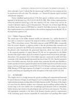
This chapter introduces a holo-extraction method of information from paper drawings, i.e. the networks
of Single Closed Regions (SCRs) of black pixels, which not only provide a unified base for recognizing
both annotations and the outlines of projections of parts, but can also build the holo-relationships
among SCRs so that it is convenient to extract lexical, syntactic and semantic information in the
subsequent phases for 3D reconstruction. Based on the holo-extraction method, this chapter further
introduces an intelligent recognition method of digital curves scanned from paper drawings for

subsequent pattern recognition and 3D reconstruction.
1. Introduction
In order to survive worldwide competition, enterprises have tried to use the computer’s huge memory
capacity, fast processing speed and user-friendly interactive graphics capabilities to automate and
tie together cumbersome and separate engineering or production tasks, including design, analysis,
Computer-Aided Intelligent Recognition Techniques and Applications Edited by M. Sarfraz
© 2005 John Wiley & Sons, Ltd
364 Holo-Extraction and Recognition of Scanned Curves
optimization,prototyping,productionplanning, tooling,orderingmaterials,programming forNumerically
Controlled (NC) machines, quality control, robot assembly and packaging. The technologies for all
these tasks rely on three-dimensional (3D) computer feature models of products made during design.
Some advancedcomputer-aided design systems have beendeveloped so that people can use thesesystems
to build 3D computer feature models for new product designs, and production without drawings has
thus appeared in some enterprises of developed countries. But enterprises have had a great deal of
two-dimensional (2D) mechanical paper drawings made in the past for their existing products, which
need to be converted to 3D computer feature models for applications. The advanced computer-aided
design systems can easily convert 3D computer models made within them into their 2D orthogonal
projections, but they cannot convert the other way round. How to convert 2D mechanical paper drawings
into 3D computer feature models is one of the major issues many enterprises are very concerned about.
In order to convert 2D mechanical paper drawings into 3D computer feature models, the 2D paper
drawings are first scanned by an optical scanner and then the scanned results are input to a computer
in the form of raster (binary) images. The conversion from the raster image to 3D model needs two
processes: understanding and 3D reconstruction. The research on the understanding process has been
implemented following three phases [1]:
1. The lexical phase. The raster image is converted into vectorized information, such as straight lines,
arcs and circles.
2. The syntactic phase. The outlines of orthographic projections of a part and the annotations are
separated; the dimension sets, including their values of both the nominal dimensions and the
tolerances, are aggregated; the crosshatching patterns are identified; and the text is recognized.
3. The semantic phase. Much semantic information needed for 3D reconstruction is obtained byfunctional

analyses of each view, including the analysis of symmetries, the recognition of technologically
meaningful entities from symbolic representation (such as bearing and threading), and so on.
After the understanding process, a 3D computer model will then be reconstructed by using geometric
matching techniques with the recognized syntactic and semantic information.
Up to now, the research on the conversion from 2D paper drawings to 3D computer feature models
has been stuck in low-level coding: essential vectorization, basic layer separation and very limited
symbol recognition [1]. One of the reasons for this is that the three phases of the understanding process
have been isolated and people have been doing their research on only one of the phases since the
whole conversion is very complicated and more difficult. For instance, the vectorization methods were
developed only for getting straight lines, arcs, circles, etc., so that much information contained in the
drawing was lost after the vectorization. Also, in some research, different methods were developed
and applied for recognizing the text and the outlines of orthographic projections of parts, respectively.
In fact, the 3D reconstruction needs not only the vectors themselves but also their relationships and
the information indicated by various symbols, from which the syntactic and semantic information can
be extracted later on. This chapter introduces a holo-extraction method of information from paper
drawings, i.e. the networks of Single Closed Regions (SCRs) of black pixels, which not only provide
a unified base for recognizing both annotations and the outlines of projections of parts, but also build
the holo-relationships among SCRs so that it is convenient to extract lexical, syntactic and semantic
information in the subsequent phases for 3D reconstruction. Based on the holo-extraction method,
this chapter further introduces an intelligent recognition method of digital curves scanned from paper
drawings for subsequent pattern recognition and 3D reconstruction.
2. Review of Current Vectorization Methods
Vectorization is a process that finds the vectors (such as straight lines, arcs and circles) from the
raster images. Much research work on this area has been done, and many vectorization methods
and their software have been developed. Although the vectorization for the lexical phase is more
Review of Current Vectorization Methods 365
mature than the technologies used for the other two higher level phases, it is yet quite far from being
perfect.
Current vectorization methods can be categorized into six types: Hough Transform (HT)-based
methods [2], thinning-based methods, contour-based methods, sparse pixel-based methods, mesh

pattern-based methods and black pixel region-based methods.
2.1 The Hough Transform-based Method
This visits each pixel of the image in the x y plane, detects peaks in its transform m c space, and
uses each peak to form a straight line defined by the following equation:
y =mx +c (19.1)
where m is its slope and c is its intercept. Since the slopes and intercepts are sampled sparsely, they
may not be as precise as the original straight lines. Moreover, this method cannot generate polylines [3].
2.2 Thinning-based Methods
Thinning is a process that applies certain algorithms to the input raster image and outputs one-pixel-
wide skeletons of black pixel regions [4–7]. Three types of algorithm have been developed, i.e. iterative
boundary erosion [5], distance transform [6] and adequate skeleton [7]. Although their speeds and
accuracies are different, they all have disadvantages: high time complexities, loss of shape information
(e.g. line width), distortions at junctions and false and spurious branches [3].
2.3 The Contour-based Method
This first finds the contour of the line object and then calculates the middle points of the pair of points
on two opposite parallel contours or edges [8–10]. Although it is much faster than thinning-based
methods and the line width is also much easier to obtain, joining up the lines for a merging junction or
a cross intersection is problematic, and it is inappropriate for use in vectorization of curved and multi-
crossing lines [3].
2.4 The Sparse Pixel-based Method
Here, the basic idea is to track the course of a one-pixel-wide ‘beam of light’, which turns orthogonally
each time when it hits the edge of the area covered by the black pixels, and to record the midpoint of
each run [11]. With some improvement based on the orthogonal zig-zag, the sparse pixel vectorization
algorithm can record the medial axis points and the width of run lengths [3].
2.5 Mesh Pattern-based Methods
These divide the entire image using a certain mesh and detect characteristic patterns by only checking
the distribution of the black pixels on the border of each unit of the mesh [12]. A control map for the
image is then prepared using these patterns. Finally, the extraction of long straight-line segments is
performed by analyzing the control map. This method not only needs a characteristic pattern database,
but also requires much more processing time. Moreover, it is not suitable for detection of more complex

line patterns, such as arcs and discontinuous (e.g. dashed or dash-dotted) lines [3].
366 Holo-Extraction and Recognition of Scanned Curves
2.6 Black Pixel Region-based Methods
These construct a semi-vector representation of a raster image first and then extract lines based on
the semi-vector representation. The semi-vector representations can be a run graph (run graph-based
methods)[13], a rectangular graph [14] or a trapezoidal graph [15]. A run is a sequence of black
pixels in either the horizontal or vertical direction. A rectangle or trapezoid consists of a certain set
of runs.
2.7 The Requirements for Holo-extraction of Information
It can be seen from the current vectorization methods that, except for black pixel region graph-based
methods, other methods are mainly focused on the speed and accuracy of generating vectors themselves,
not on holo-extraction of information. Although black pixel region graph-based methods build certain
relationships between constructed runs, rectangles or trapezoids, the regions are so small that it is
not appropriate for curve line vectorization and it is difficult to construct the relationships among
vectors.
In fact, the understanding process for its subsequent 3D reconstruction is an iterative process for
searching different level relationships and performing corresponding connections. For instance, linking
certain related pixels can form a vector. Connecting a certain set of vectors can form primitives or
characters of the text. Combining two projection lines and a dimension line containing two arrowheads
with the values for normal dimension and tolerance can produce a dimension set, which can then be
used with a corresponding primitive for parametric modeling. Aggregating the equal-spaced parallel
thin lines and the contour of their area can form a section, which can then be used with certain
section symbols for solid modeling. Connecting certain primitives referring to corresponding symbols
recognized can form certain features (e.g. bearing and threading), which can be used for feature
modeling. Matching primitives in different views according to orthogonal projective relationships can
produce a 3D model. If the primitives extracted are accurate, their projective relationships can be
determined by analyzing the coordinates of end points of these vectors. But the primitives extracted
and their projective relationships are inaccurate in paper drawings, so that this method cannot be
applied. It needs an expert system that simulates the experienced human designer’s thinking mode to
transform the inaccurate outlines of parts’ orthographic projections into 3D object images, so that their

relationships become more important and crucial. As mentioned in the first section of this chapter, the
vectorization process in the first phase should not lose the information in a drawing or the information
needed for 3D reconstruction, which are mainly different level relationships contained in the raster
image. Accordingly, a holo-extraction of information from the raster image is needed. In order to
facilitate the iterative process for searching different level relationships and performing corresponding
connections, the method needs a compact representation of the raster image as a bridge from the raster
image to understanding, which should satisfy the following requirements:
•
it can distinguish different types of linking point for different relationships of the related elements
(e.g. tangential point, intersecting point and merging junction) to provide necessary information for
extracting lexical, syntactic and semantic information in the subsequent phases;
•
it can provide a unified base for further recognizing both the outlines of orthogonal projections of
parts and the annotations, and facilitate their separation;
•
it can recognize line patterns and arrowheads, and facilitate the aggregation of related elements to
form certain syntactic information, such as dimension sets;
•
it can facilitate recognizing vectors quickly and precisely, including straight lines, arcs and circles;
•
it can provide holo-graphs of all the elements as a base for the subsequent 3D reconstruction.
The networks of SCRs reported in this chapter are developed for these purposes.
Construction of the Networks of SCRs 367
3. Construction of the Networks of SCRs
The elements and workflow of constructing the networks of SCRs are shown in Figure 19.1, and
illustrated in more detail as follows.
3.1 Generating Adjacency Graphs of Runs
Let visiting a sequence be from top to bottom for a raster image and from left to right along the
horizontal direction for each row. When visiting a row, the first black pixel converted from a white
pixel is the starting point of a run, and the last black pixel, if the next pixel is white, is the end point

of the run. The value of its end coordinates minus the starting coordinate in the horizontal direction is
its run length, the unit of which is the pixel. If the difference of two runs’ vertical coordinates is 1 and
the value of their minimal end coordinates minus maximal starting coordinates is larger than or equal
to 1, the two runs are adjacent. If A and B are adjacent and A’s vertical coordinate is larger than that
of B, A is called the predecessor of B, and B is called the successor of A. There are seven types of
run according to adjacency relationships with other runs, as shown in Figure 19.2:
By recording the adjacency relationships of runs while visiting in the assumed way, the adjacency
graphs of runs can be made using a node to represent a run, and a line between two nodes to
Raster image
Generate adjacency graphs of runs
Construct closed regions
Split closed regions into single closed regions
Build adjacency graphs of single closed regions
Construct networks of single closed regions
Figure 19.1 Elements and workflow of constructing the networks of SCRs.
(1) (2) (3) (4) (5) (6) (7)
y
x
Figure 19.2 Seven types of run. (1) Singular – has no predecessor and no successor; (2) beginning
run – has no predecessor and only one successor; (3) end run – has only one predecessor and no
successor; (4) regular run – has only one predecessor and only one successor; (5) branching run – has
one predecessor at most and more than one successor; (6) merging run – has more than one predecessor
and one successor at most; (7) cross run – has more than one predecessor and successor.