Dynamic Speech ModelsTheory, Algorithms, and Applications phần 8 ppt

P1: IML/FFX P2: IML
MOBK024-05 MOBK024-LiDeng.cls April 26, 2006 14:3
72 DYNAMIC SPEECH MODELS
The linearity between z and t as in Eq. (5.6) and Gaussianity of the target t makes the
VTR vector z(k) (at each frame k) a Gaussian as well. We now discuss the parameterization of
this Gaussian trajectory:
p(z(k) |s ) = N[z(k);μ
z(k)
, Σ
z(k)
]. (5.7)
The mean vector above is determined by the filtering function:
μ
z(k)
=
k+D

τ =k−D
c
γ
γ
|k−τ |
s (τ )
μ
T
s (τ)
= a
k
· μ
T
. (5.8)

Each f th component of vector μ
z(k)
is
μ
z(k)
( f ) =
L

l=1
a
k
(l)μ
T
(l, f ), (5.9)
where L is the total numberof phone-like HTM units as indexed byl, and f = 1, ,8 denotes
four VTR frequencies and four corresponding bandwidths.
The covariance matrix in Eq. (5.7) can be similarly derived to be
Σ
z(k)
=
k+D

τ =k−D
c
2
γ
γ
2|k−τ |
s (τ )
Σ

T
s (τ)
.
Approximating the covariance matrix by a diagonal one for each phone unit l, we represent its
diagonal elements as a vector:
σ
2
z(k)
= v
k
· σ
2
T
. (5.10)
and the target covariance matrix is also approximated as diagonal:
Σ
T
(l) ≈
⎡
⎢
⎢
⎢
⎢
⎣
σ
2
T
(l, 1) 0 ··· 0
0 σ
2

T
(l, 2) ··· 0
.
.
.
.
.
.
.
.
.
.
.
.
00··· σ
2
T
(l, 8)
⎤
⎥
⎥
⎥
⎥
⎦
.
The f th element of the vector in Eq. (5.10) is
σ
2
z(k)
( f ) =

L

l=1
v
k
(l)σ
2
T
(l, f ). (5.11)
In Eqs. (5.8) and (5.10), a
k
and v
k
are frame (k)-dependent vectors. They are constructed
for any given phone sequence and phone boundaries within the coarticulation range (2D +1
frames) centered at frame k. Any phone unit beyond the 2D +1 window contributes a zero
P1: IML/FFX P2: IML
MOBK024-05 MOBK024-LiDeng.cls April 26, 2006 14:3
MODELS WITH CONTINUOUS-VALUED HIDDEN SPEECH TRAJECTORIES 73
value to these “coarticulation” vectors’ elements. Both a
k
and v
k
are a function of the phones’
identities and temporal orders in the utterance, and are independent of the VTR dimension f .
5.1.2 Generating Acoustic Observation Data
The next generative process in the HTM provides a forward probabilistic mapping or prediction
from the stochastic VTR trajectory z(k) to the stochastic observation trajectory o(k). The
observation takes the form of linear cepstra. An analytical form of the nonlinear prediction
function F[z(k)] presented here is in the same form as described (and derived) in Section 4.2.3

of Chapter 4 and is summarized here:
F
q
(k) =
2
q
P

p=1
e
−πq
b
p
(k)
f
samp
cos(2πq
f
p
(k)
f
samp
), (5.12)
where f
samp
is the sampling frequency, P is the highest VTR order (P = 4), and q is the cepstral
order.
We now introduce the cepstral prediction’s residual vector:
r
s

(k) = o(k) −F[z(k)].
We model this residual vector as a Gaussian parameterized by residual mean vector μ
r
s (k)
and
covariance matrix Σ
r
s (k)
:
p(r
s
(k) |z(k), s) = N

r
s
(k); μ
r
s (k)
, Σ
r
s (k)

. (5.13)
Then the conditional distribution of the observation becomes:
p(o(k) |z(k), s) = N

o(k); F[z(k)] + μ
r
s (k)
, Σ

r
s (k)

. (5.14)
An alternative form of the distribution in Eq. (5.14) is the following “observation equa-
tion”:
o(k) = F[z(k)] + μ
r
s (k)
+ v
s
(k),
where the observation noise v
s
(k) ∼ N(v
s
; 0, Σ
r
s (k)
).
5.1.3 Linearizing Cepstral Prediction Function
To facilitate computing the acoustic observation (linear cepstra) likelihood, it is important to
characterize the linear cepstra uncertainty in terms of its conditional distribution on the VTR,
and to simplify the distribution to a computationally tractable form. That is, we need to specify
and approximate p(o |z, s). We take the simplest approach to linearize the nonlinear mean
P1: IML/FFX P2: IML
MOBK024-05 MOBK024-LiDeng.cls April 26, 2006 14:3
74 DYNAMIC SPEECH MODELS
function of F[z(k)] in Eq. (5.14) by using the first-order Taylor series approximation:
F[z(k)] ≈ F[z

0
(k)] +F

[z
0
(k)](z(k) − z
0
(k)), (5.15)
where the components of Jacobian matrix F

[·] can be computed in a closed form of
F

q
[ f
p
(k)] =−
4π
f
samp
e
−πq
b
p
(k)
f
samp
sin

2πq

f
p
(k)
f
samp

, (5.16)
for the VTR frequency components of z, and
F

q
[b
p
(k)] =−
2π
f
samp
e
−πq
b
p
(k)
f
samp
cos

2πq
f
p
(k)

f
samp

, (5.17)
for the VTR bandwidth components of z. In the current implementation, the Taylor series
expansion point z
0
(k) in Eq. (5.15) is taken as the tracked VTR values based on the HTM.
Substituting Eq. (5.15) into Eq. (5.14), we obtain the approximate conditional acoustic
observation probability where the mean vector μ
o
s
is expressed as a linear function of the VTR
vector z:
p(o(k) |z(k), s) ≈ N(o(k); μ
o
s
(k)
, Σ
r
s (k)
), (5.18)
where
μ
o
s (k)
= F

[z
0

(k)]z(k) +

F[z
0
(k)] −F

[z
0
(k)]z
0
(k) +μ
r
s (k)

. (5.19)
This then permits a closed-form solution for acoustic likelihood computation, which we
derive now.
5.1.4 Computing Acoustic Likelihood
An essential aspect of the HTM is its ability to provide the likelihood value for any sequence of
acoustic observation vectors o(k) in the form of cepstral parameters. The efficiently computed
likelihood provides a natural scoring mechanism comparing different linguistic hypotheses as
needed in speech recognition. No VTR values z(k) are needed in this computation as they are
treated as the hidden variables. They are marginalized (i.e., integrated over) in the linear cepstra
likelihood computation. Given the model construction and the approximation described in the
preceding section, the HTM likelihood computation by marginalization can be carried out in
P1: IML/FFX P2: IML
MOBK024-05 MOBK024-LiDeng.cls April 26, 2006 14:3
MODELS WITH CONTINUOUS-VALUED HIDDEN SPEECH TRAJECTORIES 75
a closed form. Some detailed steps of derivation give
p(o(k) |s ) =


p[o(k) |z(k), s]p[z(k) |s ] dz
≈

N[o(k); μ
o
s (k)
, Σ
r
s (k)
] N[z(k);μ
z(k)
, Σ
z(k)
] dz
= N

o(k);
¯
μ
o
s
(k)
,
¯
Σ
o
s
(k)


, (5.20)
where the time (k)-varying mean vector is
¯
μ
o
s
(k) = F[z
0
(k)] +F

[z
0
(k)][a
k
· μ
T
− z
0
(k)] +μ
r
s (k)
, (5.21)
and the time-varying covariance matrix is
¯
Σ
o
s
(k) = Σ
r
s (k)

+ F

[z
0
(k)]Σ
z
(k)(F

[z
0
(k)])
Tr
. (5.22)
The final result of Eqs. (5.20)–(5.22) are quite intuitive. For instance, when the Taylor
series expansion point is set at z
0
(k) = μ
z
(k) = a
k
· μ
T
, Eq. (5.21) is simplified to
¯
μ
o
s
(k) =
F[μ
z

(k)] +μ
r
s
, which is the noise-free part of cepstral prediction. Also, the covariance ma-
trix in Eq. (5.20) is increased by the quantity F

[z
0
(k)]Σ
z
(k)(F

[z
0
(k)])
Tr
over the covariance
matrix for the cepstral residual term Σ
r
s (k)
only. This magnitude of increase reflects the newly
introduced uncertainty in the hidden variable, measured by Σ
z
(k). The variance amplification
factor F

[z
0
(k)] results from the local “slope” in the nonlinear function F[z] that maps from
the VTR vector z(k) to cepstral vector o(k).

It is also interesting to interpret the likelihood score Eq. (5.20) as probabilistic charac-
terization of a temporally varying Gaussian process, where the time-varying mean vectors are
expressed in Eq. (5.21) and the time-varying covariance matrices are expressed in Eq. (5.22).
This may make the HTM look ostensibly like a nonstationary-state HMM (within the acoustic
dynamic model category). However, the key difference is that in HTM the dynamic structure
represented by the hidden VTR trajectory enters into the time-varying mean vector Eq. (5.21)
in two ways: (1) as the argument z
0
(k) in the nonlinear function F[z
0
(k)]; and (2) as the
term a
k
· μ
T
= μ
z(k)
in Eq. (5.21). Being closely related to the VTR tracks, they both capture
long-span contextual dependency, yet with mere context-independent VTR target parameters.
Similar properties apply to the time-varying covariance matrices in Eq. (5.22). In contrast, the
time-varying acoustic dynamic models do not have these desirable properties. For example, the
polynomial trajectory model [55, 56, 86] does regression fitting directly on the cepstral data,
exploiting no underlying speech structure and hence requiring context dependent polynomial
coefficients for representing coarticulation. Likewise, the more recent trajectory model [26] also
relies on a very large number of free model parameters to capture acoustic feature variations.
P1: IML/FFX P2: IML
MOBK024-05 MOBK024-LiDeng.cls April 26, 2006 14:3
76 DYNAMIC SPEECH MODELS
5.2 UNDERSTANDING MODEL BEHAVIOR
BY COMPUTER SIMULATION

In this section, we present the model simulation results, extracted from the work published
in [109], demonstrating major dynamic properties of the HTM. We further compare these
results with the corresponding results from direct measurements of reduction in the acoustic–
phonetic literature.
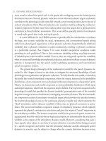
To illustrate VTR frequency or formant target undershooting, we first show the spectro-
gram of three renditions of a three-segment /iy aa iy/ (uttered by the author of this book) in
Fig. 5.1. From left to right, the speaking rate increases and speaking effort decreases, with the
durations of the /aa/’s decreasing from approximately 230 to 130 ms. Formant target under-
shooting for f
1
and f
2
is clearly visible inthe spectrogram, where automatically tracked formants
are superimposed (as the solid lines) in Fig. 5.1 to aid identification of the formant trajectories.
(The dashed lines are the initial estimates, which are then refined to give the solid lines.)
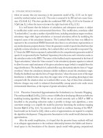
5.2.1 Effects of Stiffness Parameter on Reduction
The same kind of target undershooting for f
1
and f
2
as in Fig. 5.1 is exhibited in the model
prediction, shown in Fig. 5.2, where we also illustrate the effects of the FIR filter’s stiffness
parameter on the magnitude of formant undershooting or reduction. The model prediction
is the FIR filter’s output for f
1
and f
2
. Figs. 5.2(a)–(c) correspond to the use of the stiffness
parameter value (the same for each formant vector component) set at γ = 0.85, 0.75 and 0.65,
respectively, where in each plot the slower /iy aa iy/ sounds (with the duration of /aa/ set at

FIGURE 5.1: Spectrogram of three renditions of /iy aa iy/ by one author, with an increasingly higher
speaking rate and increasingly lower speaking efforts. The horizontal label is time, and the vertical one
is frequency
P1: IML/FFX P2: IML
MOBK024-05 MOBK024-LiDeng.cls April 26, 2006 14:3
MODELS WITH CONTINUOUS-VALUED HIDDEN SPEECH TRAJECTORIES 77
0
500
1000
1500
2000
2500
γ = [0.85], D=100
0
500
1000
1500
2000
2500
(b)
(a)
γ = [0.75]
0 20 40 60 80 100 120
0
500
1000
1500
2000
2500
(c) γ = [0.65]

Time frame (0.01 s)
f
2

(Hz)
f
1
(Hz)
/a/
/a/
/iy/
/iy/
/iy/
FIGURE 5.2: f
1
and f
2
formant or VTR frequency trajectories produced from the model for a slow /iy
aa iy/ followed by a fast /iy aa iy/. (a), (b) and (c) correspond to the use of the stiffness parameter values
of γ = 0.85, 0.75 and 0.65, respectively. The amount of formant undershooting or reduction during the
fast /aa/ is decreasing as the γ value decreases. The dashed lines indicate the formant target values and
their switch at the segment boundaries
230 ms or 23 frames) are followed by the faster /iy aa iy/ sounds (with the duration of /aa/ set
at 130 ms or 13 frames). f
1
and f
2
targets for /iy/ and /aa/ are set appropriately in the model
also. Comparing the three plots, we have the model’s quantitative prediction for the magnitude
of reduction in the faster /aa/ that is decreasing as the γ value decreases.

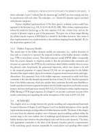
In Figs. 5.3(a)–(c), we show the same model prediction as in Fig. 5.2 but for different
sounds /iy eh iy/, where the targets for /eh/ are much closer to those of the adjacent sound /iy/
than in the previous case for /aa/. As such, the absolute amount of reduction becomes smaller.
However, the same effect of the filter parameter’s value on the size of reduction is shown as for
the previous sounds /iy aa iy/.
P1: IML/FFX P2: IML
MOBK024-05 MOBK024-LiDeng.cls April 26, 2006 14:3
78 DYNAMIC SPEECH MODELS
0
500
1000
1500
2000
2500
(a) γ = [0.85], D=100
0
500
1000
1500
2000
2500
(b) γ = [0.75]
0 20 40 60 80 100 120
0
500
1000
1500
2000
2500
(c) γ = [0.65]

Time frame
/ε/
/ε/
/iy/
/iy/
/iy/
FIGURE 5.3: Same as Fig. 5.2 except for the /iy eh iy/ sounds. Note that the f
1
and f
2
target values
for /eh/ are closer to /iy/ than those for /aa/
5.2.2 Effects of Speaking Rate on Reduction
In Fig. 5.4, we show the effects of speaking rate, measured as the inverse of the sound segment’s
duration, on the magnitude of formant undershooting. Subplots (a)–(c) correspond to three
decreasing durations of the sound /aa/ in the /iy aa iy/ sound sequence. They illustrate an
increasing amount of the reduction with the decreasing duration or increasing speaking rate.
Symbol “x” in Fig. 5.4 indicates the f
1
and f
2
formant values at the central portions of vowels/
aa/, which are predicted from the model and are used to quantify the magnitude of reduction.
These values (separately for f
1
and f
2
) for /aa/ are plotted against the inversed duration in
Fig. 5.5, together with the corresponding values for /eh/ (i.e., IPA ) in the /iy eh iy/ sound
sequence. The most interesting observation is that as the speaking rate increases, the distinction

between vowels /aa/ and /eh/ gradually diminishes if their static formant values extracted from
the dynamic patterns are used as the sole measure for the difference between the sounds. We
P1: IML/FFX P2: IML
MOBK024-05 MOBK024-LiDeng.cls April 26, 2006 14:3
MODELS WITH CONTINUOUS-VALUED HIDDEN SPEECH TRAJECTORIES 79
0
500
1000
1500
2000
2500
(a) γ = [0.85],
D
= 100
0
500
1000
1500
2000
2500
(b) γ = [0.85]
0 10 20 30 40 50 60
0
500
1000
1500
2000
2500
(c) γ = [0.85]
x

x
x
x
x
x
FIGURE 5.4: f
1
and f
2
formant trajectories produced from the model for three different durations of
/aa/ in the /iy aa iy/ sounds: (a) 25 frames (250 ms), (b) 20 frames and (c) 15 frames. The same γ value of
0.85 is used. The amount of target undershooting increases as the duration is shortened or the speaking
rate is increased. Symbol “x” indicates the f
1
and f
2
formant values at the central portions of vowels of /aa/
refer to this phenomenon as “static” sound confusion induced by increased speaking rate (or/and
by a greater degree of sloppiness in speaking).
5.2.3 Comparisons with Formant Measurement Data
The “static” sound confusion between /aa/ and /eh/ quantitatively predicted by the model
as shown in Fig. 5.5 is consistent with the formant measurement data published in [125],
where thousands of natural sound tokens were used to investigate the relationship between
the degree of formant undershooting and speaking rate. We reorganized and replotted the raw
data from [125] in Fig. 5.6, in the same formant as Fig. 5.5. While the measures of speaking
rate differ between the measurement data and model prediction and cannot be easily converted
to each other, they are generally consistent with each other. The similar trend for the greater
P1: IML/FFX P2: IML
MOBK024-05 MOBK024-LiDeng.cls April 26, 2006 14:3
80 DYNAMIC SPEECH MODELS

2 3 4 5 6 7 8 9 10
200
400
600
800
1000
1200
1400
1600
1800
2000
/ε/
Speaking rate (inverse of duration in s)
Predicted formant frequencies (Hz)
f
2
f
1

/a/
/a/
/ε/
FIGURE 5.5: Relationship, based on model prediction, between the f
1
and f
2
formant values at the
central portions of vowels and the speaking rate. Vowel /aa/ is in the carry-phrase /iy aa iy/, and vowel
/eh/ in /iy eh iy/. Note that as the speaking rate increases, the distinction between vowels /aa/ and /eh/
measured by the difference between their static formant values gradually diminishes. The same γ value

of 0.9 is used in generating all points in the figure
degree of “static” sound confusion as speaking rate increases is clearly evident from both the
measurement data (Fig. 5.6) and prediction (Fig. 5.5).
5.2.4 Model Prediction of Vocal Tract Resonance Trajectories for Real
Speech Utterances
We have used the expected VTR trajectories computed from the HTM to predict actual VTR
frequency trajectories for real speech utterances from the TIMIT database. Only the phone
identities and their boundaries are input to the model for the prediction, and no use is made of
speech acoustics. Given the phone sequence in any utterance, we first break up the compound
phones (affricates and diphthongs) into their constituents. Then we obtain the initial VTR
P1: IML/FFX P2: IML
MOBK024-05 MOBK024-LiDeng.cls April 26, 2006 14:3
MODELS WITH CONTINUOUS-VALUED HIDDEN SPEECH TRAJECTORIES 81
40 50 60 70 80 90 100 110 120
200
400
600
800
1000
1200
1400
1600
1800
2000
/ε/
Data Speaker A (Pitermann, 2000)
/ε/
/a/
/a/
f

2

f
1

Speaking rate (beat/min)
Ave. measured formant frequencies (Hz)
FIGURE 5.6: The formant measurement data from literature are reorganized and plotted, showing
similar trends to the model prediction under similar conditions
target values based on limited context dependency by table lookup (see details in [9], Ch. 13).
Then automatic and iterative target adaptation is performed for each phone-like unit based
on the difference between the results of a VTR tracker (described in [126]) and the VTR
prediction from the FIR filter model. These target values are provided not only to vowels, but
also to consonants for which the resonance frequency targets are used with weak or no acoustic
manifestation. The converged target values, together with the phone boundaries provided from
the TIMIT database, form the input to the FIR filter of the HTM and the output of the filter
gives the predicted VTR frequency trajectories.
Three example utterances from TIMIT (SI1039, SI1669 and SI2299) are shown in
Figs. 5.7–5.9. The stepwise dashed lines ( f
1
/ f
2
/ f
3
/ f
4
) are the target sequences as inputs to the
FIR filter, and the continuous lines ( f
1
/ f

2
/ f
3
/ f
4
) are the outputs of the filter as the predicted
VTR frequency trajectories. Parameters γ and D are fixed and not automatically learned. To
facilitate assessment of the accuracy in the prediction, the inputs and outputs are superimposed
P1: IML/FFX P2: IML
MOBK024-05 MOBK024-LiDeng.cls April 26, 2006 14:3
82 DYNAMIC SPEECH MODELS
Frame (10 ms)
Frequency (kHz)
γ = [0.6],
D
= 7
0 50 100 150 200 250 300 350
0
1
2
3
4
5
6
FIGURE5.7: The f
1
/ f
2
/ f
3

/ f
4
VTR frequency trajectories (smooth lines) generated from the FIR model
for VTR target filtering using the phone sequence and duration of a speech utterance (SI1039) taken from
the TIMIT database. The target sequence is shown as stepwise lines, switching at the phone boundaries
labeled in the database. They are superimposed on the utterance’s spectrogram. The utterance is “He has
never, himself, done anything for which to be hated—which of us has ”
on the spectrograms of these utterances, where the true resonances are shown as the dark
bands. For the majority of frames, the filter’s output either coincides or is close to the true VTR
frequencies, even though no acoustic information is used. Also, comparing the input and output
of the filter, we observe only a rather mild degree of target undershooting or reduction in these
and many other TIMIT utterances we have examined but not shown here.
5.2.5 Simulation Results on Model Prediction for Cepstral Trajectories
The predicted VTR trajectories in Figs. 5.7–5.9 are fed into the nonlinear mapping function
in the HTM to produce the predicted linear cepstra shown in Figs. 5.10–5.12, respectively, for