H.264 and MPEG-4 Video Compression phần 6 doc
Bạn đang xem bản rút gọn của tài liệu. Xem và tải ngay bản đầy đủ của tài liệu tại đây (479.97 KB, 31 trang )
CODING ARBITRARY-SHAPED REGIONS
•
131
Figure 5.38 Boundary MB
Figure 5.39 Boundary MB after horizontal padding
MPEG-4 VISUAL
•
132
Figure 5.40 Boundary MB after vertical padding
edge pixel. Transparent MBs are always padded after all boundary MBs have been fully
padded.
If a transparent MB has more than one neighbouring boundary MB, one of its neighbours
is chosen for extrapolation according to the following rule. If the left-hand MB is a boundary
MB, it is chosen; else if the top MB is a boundary MB, it is chosen; else if the right-hand MB
is a boundary MB, it is chosen; else the lower MB is chosen.
Transparent MBs with no nontransparent neighbours are filled with the pixel value 2
N −1
,
where N is the number of bits per pixel. If N is 8 (the usual case), these MBs are filled with
the pixel value 128.
5.4.1.3 Texture Coding in Boundary Macroblocks
The texture in an opaque MB (the pixel values in an intra-coded MB or the motion compensated
residual in an inter-coded MB) is coded by the usual process of 8 × 8 DCT, quantisation, run-
level encoding and entropy encoding (see Section 5.3.2). A boundary MB consists partly of
texture pixels (inside the boundary) and partly of undefined, transparent pixels (outside the
boundary). In a core profile object, each 8 × 8 texture block within a boundary MB is coded
using an 8 × 8 DCT followed by quantisation, run-level coding and entropy coding as usual
(see Section 7.2 for an example). (The Shape-Adaptive DCT, part of the Advanced Coding
Efficiency Profile and described in Section 5.4.3, provides a more efficient method of coding
boundary texture.)
CODING ARBITRARY-SHAPED REGIONS
•
133
Figure 5.41 Padding of transparent MB from horizontal neighbour
5.4.2 The Main Profile
A Main Profile CODEC supports Simple and Core objects plus Scalable Texture objects (see
Section 5.6.1) and Main objects. The Main object adds the following tools:
r
interlace (described in Section 5.3.3);
r
object-based coding with grey (‘alpha plane’) shape;
r
Sprite coding.
In theCore Profile, object shape is specified bya binaryalpha mask such that each pixel position
is marked as ‘opaque’ or ‘transparent’. The Main Profile adds support for grey shape masks,
in which each pixel position can take varying levels of transparency from fully transparent to
fully opaque. This is similar to the concept of Alpha Planes used in computer graphics and
allows the overlay of multiple semi-transparent objects in a reconstructed (rendered) scene.
Sprite coding is designed to support efficient coding of background objects. In many
video scenes, the background does not change significantly and those changes that do occur
are often due to camera movement. A ‘sprite’ is a video object (such as the scene background)
that is fully or partly transmitted at the start of a scene and then may change in certain limited
ways during the scene.
5.4.2.1 Grey Shape Coding
Binary shape coding (described in Section 5.4.1.1) has certain drawbacks in the representation
of video scenes made up of multiple objects. Objects or regions in a ‘natural’ video scene
may be translucent (partially transparent) but binary shape coding only supports completely
transparent (‘invisible’) or completely opaque regions. It is often difficult or impossible to
segment video objects neatly (since object boundaries may not exactly correspond with pixel
positions), especially when segmentation is carried out automatically or semi-automatically.
MPEG-4 VISUAL
•
134
Figure 5.42 Grey-scale alpha mask for boundary MB
Figure 5.43 Boundary MB with grey-scale transparency
For example, the edge of the VOP shown in Figure 5.30 is not entirely ‘clean’ and this may
lead to unwanted artefacts around the VOP edge when it is rendered with other VOs.
Grey shape coding gives more flexible control of object transparency. A grey-scale alpha
plane is coded for each macroblock, in which each pixel position has a mask value between
0 and 255, where 0 indicates that the pixel position is fully transparent, 255 indicates that it
is fully opaque and other values specify an intermediate level of transparency. An example
of a grey-scale mask for a boundary MB is shown in Figure 5.42. The transparency ranges
from fully transparent (black mask pixels) to opaque (white mask pixels). The rendered MB
is shown in Figure 5.43 and the edge of the object now ‘fades out’ (compare this figure
with Figure 5.32). Figure 5.44 is a scene constructed of a background VO (rectangular) and
two foreground VOs. The foreground VOs are identical except for their transparency, the
left-hand VO uses a binary alpha mask and the right-hand VO has a grey alpha mask which
helps the right-hand VO to blend more smoothly with the background. Other uses of grey
shape coding include representing translucent objects, or deliberately altering objects to make
them semi-transparent (e.g. the synthetic scene in Figure 5.45).
CODING ARBITRARY-SHAPED REGIONS
•
135
Figure 5.44 Video scene with binary-alpha object (left) and grey-alpha object (right)
Figure 5.45 Video scene with semi-transparent object
Grey scale alpha masks are coded using two components, a binary support mask that
indicates which pixels are fully transparent (external to the VO) and which pixels are semi-
or fully-opaque (internal to the VO), and a grey scale alpha plane. Figure 5.33 is the binary
support mask for the grey-scale alpha mask of Figure 5.42. The binary support mask is coded
in the same way as a BAB (see Section 5.4.1.1). The grey scale alpha plane (indicating the
level of transparency of the internal pixels) is coded separately in the same way as object
texture (i.e. each 8 × 8 block within the alpha plane is transformed using the DCT, quantised,
MPEG-4 VISUAL
•
136
Figure 5.46 Sequence of frames
reordered, run-level and entropy coded). The decoder reconstructs the grey scale alpha plane
(which may not be identical to the original alpha plane due to quantisation distortion) and the
binary support mask. If the binary support mask indicates that a pixel is outside the VO, the
corresponding grey scale alpha plane value is set to zero. In this way, the object boundary is
accurately preserved (since the binary support mask is losslessly encoded) whilst the decoded
grey scale alpha plane (and hence the transparency information) may not be identical to the
original.
The increased flexibility provided by grey scale alpha shape coding is achieved at a cost
of reduced compression efficiency. Binary shape coding requires the transmission of BABs
for each boundary MB and in addition, grey scale shape coding requires the transmission of
grey scale alpha plane data for every MB that is semi-transparent.
5.4.2.2 Static Sprite Coding
Three frames from a video sequence are shown in Figure 5.46. Clearly, the background does not
change during the sequence (the camera position is fixed). The background (Figure 5.47) may
be coded as a static sprite. A static sprite is treated as a texture image that may move or warp
in certain limited ways, in order to compensate for camera changes such as pan, tilt, rotation
and zooming. In a typical scenario, a sprite may be much larger than the visible area of the
scene. As the camera ‘viewpoint’ changes, the encoder transmits parameters indicating how
the sprite should be moved and warped to recreate the appropriate visible area in the decoded
scene. Figure 5.48 shows a background sprite (the large region) and the area viewed by the
camera at three different points in time during a video sequence. As the sequence progresses,
the sprite is moved, rotated and warped so that the visible area changes appropriately. A sprite
may have arbitrary shape (Figure 5.48) or may be rectangular.
The use of static sprite coding is indicated by setting sprite
enable to ‘Static’ in a VOL
header, after which static sprite coding is used throughout the VOP. The first VOP in a static
sprite VOL is an I-VOP and this is followed by a series of S-VOPs (Static Sprite VOPs). Note
that a Static Sprite S-VOP is coded differently from a Global Motion Compensation S(GMC)-
VOP (described in Section 5.3.3).There are two methods of transmitting and manipulating
sprites, a ‘basic’ sprite (sent in its entirety at the start of a sequence) and a ‘low-latency’ sprite
(updated piece by piece during the sequence).
CODING ARBITRARY-SHAPED REGIONS
•
137
Figure 5.47 Background sprite
background sprite
1
2
3
Figure 5.48 Background sprite and three different camera viewpoints
Basic Sprite
The first VOP (I-VOP) contains the entire sprite, encoded in the same way as a ‘normal’
I-VOP. The sprite may be larger than the visible display size (to accommodate camera move-
ments during the sequence). At the decoder, the sprite is placed in a Sprite Buffer and is not
immediately displayed. All further VOPs in the VOL are S-VOPs. An S-VOP contains up
to four warping parameters that are used to move and (optionally) warp the contents of the
Sprite Buffer in order to produce the desired background display. The number of warping
parameters per S-VOP (up to four) is chosen in the VOL header and determines the flexibility
of the Sprite Buffer transformation. A single parameter per S-VOP enables linear transla-
tion (i.e. a single motion vector for the entire sprite), two or three parameters enable affine
MPEG-4 VISUAL
•
138
transformation of the sprite (e.g. rotation, shear) and four parameters enable a perspective
transform.
Low-latency sprite
Transmitting an entire sprite in Basic Sprite mode at the start of a VOL may introduce sig-
nificant latency because the sprite may be much larger than an individual displayed VOP.
The Low-Latency Sprite mode enables an encoder to send initially a minimal size and/or low-
quality version of the sprite and then update it during transmission of the VOL. The first I-VOP
contains part or all of the sprite (optionally encoded at a reduced quality to save bandwidth)
together with the height and width of the entire sprite.
Each subsequent S-VOP may contain warping parameters (as in the Basic Sprite mode)
and one or more sprite ‘pieces’. A sprite ‘piece’ covers a rectangular area of the sprite and
contains macroblock data that (a) constructs part of the sprite that has not previously been
decoded (‘static-sprite-object’ piece) or (b) improves the quality of part of the sprite that
has been previously decoded (‘static-sprite-update’ piece). Macroblocks in a ‘static-sprite-
object’ piece are encoded as intra macroblocks (including shape information if the sprite is not
rectangular). Macroblocks in a ‘static-sprite-update’ piece are encoded as inter macroblocks
using forward prediction from the previous contents of the sprite buffer (but without motion
vectors or shape information).
Example
The sprite shown in Figure 5.47 is to be transmitted in low-latency mode. The initial I-VOP
contains a low-quality version of part of the sprite and Figure 5.49 shows the contents of the
sprite buffer after decoding the I-VOP. An S-VOP contains a new piece of the sprite, encoded in
high-quality mode (Figure 5.50) and this extends the contents of the sprite buffer (Figure 5.51).
A further S-VOP contains a residual piece (Figure 5.52) that improves the quality of the top-left
part of the current sprite buffer. After adding the decoded residual, the sprite buffer contents are
as shown Figure 5.53. Finally, four warping points are transmitted in a further S-VOP to produce
a change of rotation and perspective (Figure 5.54).
5.4.3 The Advanced Coding Efficiency Profile
The ACE profile is a superset of the Core profile that supports coding of grey-alpha video
objects with high compression efficiency. In addition to Simple and Core objects, it includes
the ACE object which adds the following tools:
r
quarter-pel motion compensation (Section 5.3.3);
r
GMC (Section 5.3.3);
r
interlace (Section 5.3.3);
r
grey shape coding (Section 5.4.2);
r
shape-adaptive DCT.
The Shape-Adaptive DCT (SA-DCT) is based on pre-defined sets of one-dimensional DCT
basis functions and allows an arbitrary region of a block to be efficiently transformed and
compressed. The SA-DCT is only applicable to 8 × 8 blocks within a boundary BAB that
CODING ARBITRARY-SHAPED REGIONS
•
139
Figure 5.49 Low-latency sprite: decoded I-VOP
Figure 5.50 Low-latency sprite: static-sprite-object piece
Figure 5.51 Low-latency sprite: buffer contents (1)
Figure 5.52 Low-latency sprite: static-sprite-update piece
Figure 5.53 Low-latency sprite: buffer contents (2)
Figure 5.54 Low-latency sprite: buffer contents (3)
CODING ARBITRARY-SHAPED REGIONS
•
141
Residual X Residual X
Intermediate Y Intermediate Y Coefficients Z
Shift
vertically
1-D column
DCT
Shift
horizontally
1-D row
DCT
Figure 5.55 Shape-adaptive DCT
Fine Granular
Scalability
Core Scalable
Simple
Scalable
Core
Simple
Interlace
B-VOP
Alternate Quant
FGS
FGS Temporal
Scalability
Temporal
Scalability
(rectangular)
Spatial Scalability
(rectangular)
Object-based
spatial scalability
I-VOP
P-VOP
4MV
UMV
Intra Pred
Video packets
Data Partitioning
RVLCs
B-VOP
Temporal
Scalability
(rectangular)
Spatial Scalability
(rectangular)
Figure 5.56 Tools and objects for scalable coding
contain one or more transparent pixels. The Forward SA-DCT consists of the following steps
(Figure 5.55):
1. Shift opaque residual values X to the top of the 8 × 8 block.
2. Apply a 1D DCT to each column (the number of points in the transform matches the number
of opaque values in each column).
3. Shift the resulting intermediate coefficients Y to the left of the block.
4. Apply a 1D DCT to each row (matched to the number of values in each row).
The final coefficients (Z) are quantised, zigzag scanned and encoded. The decoder reverses
the process (making use of the shape information decoded from the BAB) to reconstruct the
8 × 8 block of samples. The SA-DCT is more complex than the normal 8 × 8 DCT but can
improve coding efficiency for boundary MBs.
5.4.4 The N-bit Profile
The N-bit profile contains Simple and Core objects plus the N-bit tool. This supports coding of
luminance and chrominance data containing between four and twelve bits per sample (instead
of the usual restriction to eight bits per sample). Possible applications of the N-bit profile
include video coding for displays with low colour depth (where the limited display capability
means that less than eight bits are required to represent each sample) or for high-quality display
applications (where the display has a colour depth of more than eight bits per sample and high
coded fidelity is desired).
MPEG-4 VISUAL
•
142
video
sequence
encoder
base layer
enhancement
layer 1
enhancement
layer N
decoder A
decoder B
basic-quality
sequence
high-quality
sequence
Figure 5.57 Scalable coding: general concept
5.5 SCALABLE VIDEO CODING
Scalable encoding of video data enables a decoder to decode selectively only part of the coded
bitstream. The coded stream is arranged in a number of layers, including a ‘base’ layer and
one or more ‘enhancement’ layers (Figure 5.57). In this figure, decoder A receives only the
base layer and can decode a ‘basic’ quality version of the video scene, whereas decoder B
receives all layers and decodes a high quality version of the scene. This has a number of
applications, for example, a low-complexity decoder may only be capable of decoding the
base layer; a low-rate bitstream may be extracted for transmission over a network segment
with limited capacity; and an error-sensitive base layer may be transmitted with higher priority
than enhancement layers.
MPEG-4 Visual supports a number of scalable coding modes. Spatial scalability enables
a (rectangular) VOP to be coded at a hierarchy of spatial resolutions. Decoding the base
layer produces a low-resolution version of the VOP and decoding successive enhancement
layers produces a progressively higher-resolution image. Temporal scalability provides a low
frame-rate base layer and enhancement layer(s) that build up to a higher frame rate. The
standard also supports quality scalability, in which the enhancement layers improve the visual
quality of the VOP and complexity scalability, in which the successive layers are progressively
more complex to decode. Fine Grain Scalability (FGS) enables the quality of the sequence
to be increased in small steps. An application for FGS is streaming video across a network
connection, in which it may be useful to scale the coded video stream to match the available
bit rate as closely as possible.
5.5.1 Spatial Scalability
The base layer contains a reduced-resolution version of each coded frame. Decoding the
base layer alone produces a low-resolution output sequence and decoding the base layer with
enhancement layer(s) produces a higher-resolution output. The following steps are required
to encode a video sequence into two spatial layers:
1. Subsample eachinput video frame (Figure 5.58) (orvideo object) horizontally and vertically
(Figure 5.59).
2. Encode the reduced-resolution frame to form the base layer.
3. Decode the base layer and up-sample to the original resolution to form a prediction frame
(Figure 5.60).
4. Subtract the full-resolution frame from this prediction frame (Figure 5.61).
5. Encode the difference (residual) to form the enhancement layer.
SCALABLE VIDEO CODING
•
143
Figure 5.58 Original video frame
Figure 5.59 Sub-sampled frame to be encoded as base layer
Figure 5.60 Base layer frame (decoded and upsampled)
MPEG-4 VISUAL
•
144
Figure 5.61 Residual to be encoded as enhancement layer
A single-layer decoder decodes only the base layer to produce a reduced-resolution output
sequence. A two-layer decoder can reconstruct a full-resolution sequence as follows:
1. Decode the base layer and up-sample to the original resolution.
2. Decode the enhancement layer.
3. Add the decoded residual from the enhancement layer to the decoded base layer to form
the output frame.
An I-VOP in an enhancement layer is encoded without any spatial prediction, i.e. as a complete
frame or object at the enhancement resolution. In an enhancement layer P-VOP, the decoded,
up-sampled base layer VOP (at the same position in time) is used as a prediction without any
motion compensation. The difference between this prediction and the input frame is encoded
using the texture coding tools, i.e. no motion vectors are transmitted for an enhancement
P-VOP. An enhancement layer B-VOP is predicted from two directions. The backward pre-
diction is formed by the decoded, up-sampled base layer VOP (at the same position in time),
without any motion compensation (and hence without any MVs). The forward prediction is
formed by the previous VOP in the enhancement layer (even if this is itself a B-VOP), with
motion-compensated prediction (and hence MVs).
If the VOP has arbitrary (binary) shape, a base layer and enhancement layer BAB is
required for each MB. The base layer BAB is encoded as usual, based on the shape and size of
the base layer object. A BAB in a P-VOP enhancement layer is coded using prediction from
an up-sampled version of the base layer BAB. A BAB in a B-VOP enhancement layer may be
coded in the same way, or using forward prediction from the previous enhancement VOP (as
described in Section 5.4.1.1).
5.5.2 Temporal Scalability
The base layer of a temporal scalable sequence is encoded at a low video frame rate and a
temporal enhancement layer consists of I-, P- and/or B-VOPs that can be decoded together
with the base layer to provide an increased video frame rate. Enhancement layer VOPs are
predicted using motion-compensated prediction according to the following rules.
SCALABLE VIDEO CODING
•
145
1
20
3
enhancement
layer VOPs
base layer
VOPs
(i)
(ii) (iii)
Figure 5.62 Temporal enhancement P-VOP prediction options
1
20
(i)
(ii)
20
3 1
2
3
(iii)
Figure 5.63 Temporal enhancement B-VOP prediction options
An enhancement I-VOP is encoded without any prediction. An enhancement P-VOP is
predicted from (i) the previous enhancement VOP, (ii) the previous base layer VOP or (iii) the
next base layer VOP (Figure 5.62). An enhancement B-VOP is predicted from (i) the previous
enhancement and previous base layer VOPs, (ii) the previous enhancement and next base layer
VOPs or (iii) the previous and next base layer VOPs (Figure 5.63).
5.5.3 Fine Granular Scalability
Fine Granular Scalability (FGS) [5] is a method of encoding a sequence as a base layer and
enhancement layer. The enhancement layer can be truncated during or after encoding (reducing
the bitrate and the decoded quality) to give highly flexible control over the transmitted bitrate.
FGS may be useful for video streaming applications, in which the available transmission
bandwidth may not be known in advance. In a typical scenario, a sequence is coded as a base
layer and a high-quality enhancement layer. Upon receiving a request to send the sequence at
a particular bitrate, the streaming server transmits the base layer and a truncated version of the
enhancement layer. The amount of truncation is chosen to match the available transmission
bitrate, hence maximising the quality of the decoded sequence without the need to re-encode
the video clip.
MPEG-4 VISUAL
•
146
Texture
FDCT Quant
Rescale
Encode
each
bitplane
Encode
coefficients
+
-
Base
layer
Enhancement
layer
Figure 5.64 FGS encoder block diagram (simplified)
13 -11
17
-3
0 0
00
0
0
Figure 5.65 Block of residual coefficients (top-left corner)
Encoding
Figure 5.64 shows a simplified block diagram of an FGS encoder (motion compensation is
not shown). In the Base Layer, the texture (after motion compensation) is transformed with
the forward DCT, quantised and encoded. The quantised coefficients are re-scaled (‘inverse
quantised’) and these re-scaled coefficients are subtracted from the unquantised DCT coeffi-
cients to give a set of difference coefficients. The difference coefficients for each block are
encoded as a series of bitplanes. First, the residual coefficients are reordered using a zigzag
scan. The highest-order bits of each coefficient (zeros or ones) are encoded first (the MS bit-
plane) followed by the next highest-order bits and so on until the LS bits have been encoded.
Example
A block of residual coefficients is shown in Figure 5.65 (coefficients not shown are zero). The
coefficients are reordered in a zigzag scan to produce the following list:
+13, −11, 0, 0, +17, 0, 0, 0, −3, 0, 0
The bitplanes correspondingto the magnitudeof eachresidual coefficient are shown in Table 5.6. In
this case, the highest plane containing nonzero bits is plane 4 (because the highest magnitude is 17).
SCALABLE VIDEO CODING
•
147
Table 5.6 Residual coefficient bitplanes (magnitude)
Value +13 −1100+17000−3 0
Plane 4 (MSB) 0 0 0 0 1 0 0 0 0 0
Plane 3 1 1 0 0 0 0 0 0 0 0
Plane 2 1 1 0 0 0 0 0 0 0 0
Plane 1 0 0 0 0 0 0 0 0 1 0
Plane 0 (LSB) 1 1 0 0 1 0 0 0 1 0
Table 5.7 Encoded values
Plane Encoded values
4 (4, EOP) (+)
3 (0) (+) (0, EOP) (−)
2 (0, EOP)
1 (1) (6, EOP) (−)
0 (0) (0) (2) (3, EOP)
Each bitplane contains a series of zeros and ones. The ones are encoded as (run, EOP) where
‘EOP’ indicates ‘end of bitplane’ and each (run, EOP) pair is transmitted as a variable-length
code. Whenever the MS bit of a coefficient is encoded, it is immediately followed in the bitstream
by a sign bit. Table 5.7 lists the encoded values for each bitplane. Bitplane 4 contains four zeros,
followed by a 1. This is the last nonzero bit and so is encoded as (4, EOP). This also the MS bit
of the coefficient ‘+17’ and so the sign of this coefficient is encoded.
This example illustrates the processing of one block. The encoding procedure for a
complete frame is as follows:
1. Find the highest bit position of any difference coefficient in the frame (the MSB).
2. Encode each bitplane as described above, starting with the plane containing the MSB.
Each complete encoded bitplane is preceded by a start code, making it straightforward
to truncate the bitstream by sending only a limited number of encoded bitplanes.
Decoding
The decoder decodes the base layer and enhancement layer (which may be truncated).
The difference coefficients are reconstructed from the decoded bitplanes, added to the base
layer coefficients and inverse transformed to produce the decoded enhancement sequence
(Figure 5.66).
If the enhancement layer has been truncated, then the accuracy of the difference coef-
ficients is reduced. For example, assume that the enhancement layer described in the above
example is truncated after bitplane 3. The MS bits (and the sign) of the first three nonzero
coefficients are decoded (Table 5.8); if the remaining (undecoded) bitplanes are filled with
MPEG-4 VISUAL
•
148
Table 5.8 Decoded values (truncated after plane 3)
Plane 4 (MSB) 0 0 0 0 1 00000
Plane 3 1 1 0 0 000000
Plane 2 0 0 0 0 000000
Plane 1 0 0 0 0 000000
Plane 0 (LSB) 0 0 0 0 000000
Decoded value +8 −800+1600000
Decode
coefficients
Rescale IDCT
Decode
bitplanes
+
+
IDCT
Base
layer
Enhancement
layer (may be
truncated)
Texture
(base layer)
Texture
(enhancement
layer)
Figure 5.66 FGS decoder block diagram (simplified)
zeros then the list of output values becomes:
+8, −8, 0, 0, +16, 0
Optional enhancements to FGScoding includeselective enhancement (in which bit planes
of selected MBs are bit-shifted up prior to encoding, in order to give them a higher priority and
a higher probability of being included in a truncated bitstream) and frequency weighting (in
which visually-significant low frequency DCT coefficients are shifted up prior to encoding,
again in order to give them higher priority in a truncated bitstream).
5.5.4 The Simple Scalable Profile
The Simple Scalable profile supports Simple and Simple Scalable objects. The Simple Scalable
object contains the following tools:
r
I-VOP, P-VOP, 4MV, unrestricted MV and Intra Prediction;
r
Video packets, Data Partitioning and Reversible VLCs;
r
B-VOP;
r
Rectangular Temporal Scalability (1 enhancement layer) (Section 5.5.2);
r
Rectangular Spatial Scalability (1 enhancement layer) (Section 5.5.1).
The last two tools support scalable coding of rectangular VOs.
5.5.5 The Core Scalable Profile
The Core Scalable profile includes Simple, Simple Scalable and Core objects, plus the Core
Scalable object which features the following tools, in each case with up to two enhancement
layers per object:
TEXTURE CODING
•
149
r
Rectangular Temporal Scalability (Section 5.5.2);
r
Rectangular Spatial Scalability (Section 5.5.1);
r
Object-based Spatial Scalability (Section 5.5.1).
5.5.6 The Fine Granular Scalability Profile
The FGS profile includes Simple and Advanced Simple objects plus the FGS object which
includes these tools:
r
B-VOP, Interlace and Alternate Quantiser tools;
r
FGS Spatial Scalability;
r
FGS Temporal Scalability.
FGS ‘Spatial Scalability’ uses the encoding and decoding techniques described in Section
5.5.3 to encode each frame as a base layer and an FGS enhancement layer. FGS ‘Tempo-
ral Scalability’ combines FGS (Section 5.5.3) with temporal scalability (Section 5.5.2). An
enhancement-layer frame is encoded using forward or bidirectional prediction from base layer
frame(s) only. The DCT coefficients of the enhancement-layer frame are encoded in bitplanes
using the FGS technique.
5.6 TEXTURE CODING
The applications targeted by the developers of MPEG4 include scenarios where it is necessary
to transmit still texture (i.e. still images). Whilst block transforms such as the DCT are widely
considered to be the best practical solution for motion-compensated video coding, the Discrete
Wavelet Transform (DWT) is particularly effective for coding still images (see Chapter 3) and
MPEG-4 Visual uses the DWT as the basis for tools to compress still texture. Applications
include the coding of rectangular texture objects (such as complete image frames), coding of
arbitrary-shaped texture regions and coding of texture to be mapped onto animated 2D or 3D
meshes (see Section 5.8).
The basic structure of a still texture encoder is shown in Figure 5.68. A 2D DWT is
applied to the texture object, producing a DC component (low-frequency subband) and a
number of AC (high-frequency) subbands (see Chapter 3). The DC subband is quantised, pre-
dictively encoded (using a form of DPCM) and entropy encoded using an arithmetic encoder.
The AC subbands are quantised and reordered (‘scanned’), zero-tree encoded and entropy
encoded.
Discrete Wavelet Transform
The DWT adopted for MPEG-4 Still Texture coding is the Daubechies (9,3)-tap biorthogonal
filter [6]. This is essentially a matched pair of filters, one low pass (with three filter coefficients
or ‘taps’) and one high pass (with nine filter taps).
Quantisation
The DC subband is quantised using a scalar quantiser (see Chapter 3). The AC subbands may
be quantised in one of three ways:
MPEG-4 VISUAL
•
150
Advanced
Scalable
Texture
Scalable still
texture
Scalable
Texture
Scalable shape
coding
Texture error
resilience
Wavelet tiling
Figure 5.67 Tools and objects for texture coding
DWT
Quant
Predictive
coding
Quant and
Scanning
Zero-tree
coding
Arithmetic
encoder
Still
texture
DC subband
AC subbands
Coded
bitstream
Figure 5.68 Wavelet still texture encoder block diagram
1. Scalar quantisation using a single quantiser (‘mode 1’), prior to reordering and zero-tree
encoding.
2. ‘Bilevel’ quantisation (‘mode 3’) after reordering. The reordered coefficients are coded one
bitplane at a time (see Section 5.5.3 for a discussion of bitplanes) using zero-tree encoding.
The coded bitstream can be truncated at any point to provide highly scalable decoding (in
a similar way to FGS, see previous section).
3. ‘Multilevel’ quantisation (‘mode 2’) prior to reordering and zero-tree encoding. A series
of quantisers are applied, from coarse to fine, with the output of each quantiser forming a
series of layers (a type of scalable coding).
Reordering
The coefficients of the AC subbands are scanned or reordered in one of two ways:
1. Tree-order. A ‘parent’ coefficient in the lowest subband is coded first, followed by its
‘child’ coefficients in the next higher subband, and so on. This enables the EZW coding
(see below) to exploit the correlation between parent and child coefficients. The first three
trees to be coded in a set of coefficients are shown in Figure 5.69.
TEXTURE CODING
•
151
DC
1st tree
2nd tree 3rd tree
Figure 5.69 Tree-order scanning
DC
1st band 2nd band 3rd band
Figure 5.70 Band-by-band scanning
2. Band-by-band order. All the coefficients in the first AC subband are coded, followed by all
the coefficients in the next subband, and so on (Figure 5.70). This scanning method tends to
reduce coding efficiency but has the advantage that it supports a form of spatial scalability
since a decoder can extract a reduced-resolution image by decoding a limited number of
subbands.
DC Subband Coding
The coefficients in the DC subband are encoded using DPCM. Each coefficient is spatially
predicted from neighbouring, previously-encoded coefficients.
MPEG-4 VISUAL
•
152
Table 5.9 Zero-tree coding symbols
Symbol Meaning
ZeroTree Root (ZTR) The current coefficient and all subsequent coefficients in the tree
(or band) are zero. No further data is coded for this tree (or band).
Value + ZeroTree Root The current coefficient is nonzero but all subsequent coefficients are
(VZTR) zero. No further data is coded for this tree/band.
Value (VAL) The current coefficient is nonzero and one or more subsequent
coefficients are nonzero. Further data must be coded.
Isolated Zero (IZ) The current coefficient is zero but one or more subsequent coefficients
are nonzero. Further data must be coded.
AC Subband Coding
Coding of coefficients in the AC subbands is based on EZW (Embedded Zerotree Wavelet
coding). The coefficients of each tree (or each subband if band-by-band scanning is used) are
encoded starting with the first coefficient (the ‘root’ of the tree if tree-order scanning is used)
and each coefficient is coded as one of the four symbols listed in Table 5.9.
Entropy Coding
The symbols produced by the DC and AC subband encoding processes are entropy coded
using a context-based arithmetic encoder. Arithmetic coding is described in Chapter 3 and the
principle of context-based arithmetic coding is discussed in Section 5.4.1 and Chapter 6.
5.6.1 The Scalable Texture Profile
The Scalable Texture Profile contains just one object which in turn contains one tool, Scalable
Texture. This tool supports the coding process described in the preceding section, for rectan-
gular video objects only. By selecting the scanning mode and quantiser method it is possible
to achieve several types of scalable coding.
(a) Single quantiser, tree-ordered scanning: no scalability.
(b) Band-by-band scanning: spatial scalability (by decoding a subset of the bands).
(c) Bilevel quantiser: bitplane-based scalability, similar to FGS.
(d) Multilevel quantiser: ‘quality’ scalability, with one layer per quantiser.
5.6.2 The Advanced Scalable Texture Profile
The Advanced Scalable Texture profile contains the Advanced Scalable Texture object which
adds extra tools to Scalable Texture. Wavelet tiling enables an image to be divided into several
nonoverlapping sub-images or ‘tiles’, each coded using the wavelet texture coding process
described above. This tool is particularly useful for CODECs with limited memory, since
the wavelet transform and other processing steps can be applied to a subset of the image
at a time. The shape coding tool adds object-based capabilities to the still texture coding
process by adapting the DWT to deal with arbitrary-shaped texture objects. Using the error
CODING STUDIO-QUALITY VIDEO
•
153
Core Studio
Simple Studio
P-VOP
Frame/Field
I-VOP
Interlace
Studio Slice
Studio DPCM
Studio Binary and
Gray Shape
Studio Sprite
Figure 5.71 Tools and objects for studio coding
resilience tool, the coded texture is partitioned into packets (‘texture packets’). The bitstream
is processed in Texture Units (TUs), each containing a DC subband, a complete coded tree
structure (tree-order scanning) or a complete coded subband (band-by-band scanning). A
texture packet contains one or more coded TUs. This packetising approach helps to minimise
the effect of a transmission error by localising it to one decoded TU.
5.7 CODING STUDIO-QUALITY VIDEO
Before broadcasting digital video to the consumer it is necessary to code (or transcode) the
material into a compressed format. In order to maximise the quality of the video delivered to
the consumer it is important to maintain high quality during capture, editing and distribution
between studios. The Simple Studio and Core Studio profiles of MPEG-4 Visual are designed
to support coding of video at a very high quality for the studio environment. Important con-
siderations include maintaining high fidelity (with near-lossless or lossless coding), support
for 4:4:4 and 4:2:2 colour depths and ease of transcoding (conversion) to/from legacy formats
such as MPEG-2.
5.7.1 The Simple Studio Profile
The Simple Studio object is intended for use in the capture, storage and editing of high quality
video. It supports only I-VOPs (i.e. no temporal prediction) and the coding process is modified
in a number of ways.
Source format: The Simple Studio profile supports coding of video sampled in 4:2:0, 4:2:2 and
4:4:4 YCbCr formats (see Chapter 2 for details of these sampling modes) with progressive
MPEG-4 VISUAL
•
154
10
2 3
4
6
5
7
10
2 3
4
6
5
7
8
10 11
9
YCbCr
YCbCr
4:4:4 macroblock structure (12 blocks)
Figure 5.72 Modified macroblock structures (4:2:2 and 4:4:4 video)
1
5
etc
0
2
4
3
8
7
6
9
Figure 5.73 Example slice structure
or interlaced scanning. The modified macroblock structures for 4:2:2 and 4:4:4 video are
shown in Figure 5.72.
Transform and quantisation: The precision of the DCT and IDCT are extended by three frac-
tional bits. Together with modifications to the forward and inverse quantisation processes,
this enables fully lossless DCT-based encoding and decoding. In some cases, lossless DCT
coding of intra data may result in a coded frame that is larger than the original and for this
reason the encoder may optionally use DPCM to code the frame data instead of the DCT
(see Chapter 3).
Shape coding: Binary shape information is coded using PCM rather than arithmetic coding
(in order to simplify the encoding and decoding process). Alpha (grey) shape may be coded
with an extended resolution of up to 12 bits.
Slices: Coded data are arranged in slices in a similar way to MPEG-2 coded video [7]. Each
slice includes a start code and a series of coded macroblocks and the slices are arranged
in raster order to cover the coded picture (see for example Figure 5.73). This structure is
adopted to simplify transcoding to/from an MPEG-2 coded representation.
VOL headers: Additional data fields are added to the VOL header, mimicking those in an
MPEG-2 picture header in order to simplify MPEG-2 transcoding.
CODING SYNTHETIC VISUAL SCENES
•
155
Simple Face
Facial Animation
Parameters
Basic
Animated
Texture
Animated 2D
Mesh
Simple FBA
Body Animation
Parameters
Scalable still
texture
Binary Shape
2D dynamic mesh
(uniform topology)
Core
2D dynamic mesh
(Delaunay
topology)
Figure 5.74 Tools and objects for animation
5.7.2 The Core Studio Profile
The Core Studio object is intended for distribution of studio-quality video (for example be-
tween production studios) and adds support for Sprites and P-VOPs to the Simple Studio
tools. Sprite coding is modified by adding extra sprite control parameters that closely mimic
the properties of ‘real’ video cameras, such as lens distortion. Motion compensation and mo-
tion vector coding in P-VOPs is modified for compatibility with the MPEG-2 syntax, for
example, motion vectors are predictively coded using the MPEG-2 method rather than the
usual MPEG-4 median prediction method.
5.8 CODING SYNTHETIC VISUAL SCENES
For the first time in an international standard, MPEG4 introduced the concept of ‘hybrid’
synthetic and natural video objects for visual communication. According to this concept,
some applications may benefit from using a combination of tools from the video coding
community (designed for coding of ‘real world’ or ‘natural’ video material) and tools from
the 2D/3D animation community (designed for rendering ‘synthetic’ or computer-generated
visual scenes).
MPEG4 Visual includes several tools and objects that can make use of a combination
of animation and natural video processing (Figure 5.74). The Basic Animated Texture and
Animated 2D Mesh object types support the coding of 2D meshes that represent shape and
motion, together with still texture that may be mapped onto a mesh. A tool for representing
and coding 3D Mesh models is included in MPEG-4 Visual Version 2 but is not yet part of any
profile. The Face and Body Animation tools enable a human face and/or body to be modelled
and coded [8].
It has been shown that animation-based tools have potential applications to very low bit
rate video coding [9]. However, in practice, the main application of these tools to date has
been in coding synthetic (computer-generated) material. As the focus of this book is natural
video coding, these tools will not be covered in detail.
5.8.1 Animated 2D and 3D Mesh Coding
A 2D mesh is made up of triangular patches and covers the 2D plane of an image or VO. De-
formation or motion between VOPs can be modelled by warping the triangular patches. A 3D