H.264 and MPEG-4 Video Compression phần 8 docx
Bạn đang xem bản rút gọn của tài liệu. Xem và tải ngay bản đầy đủ của tài liệu tại đây (222.92 KB, 31 trang )
THE BASELINE PROFILE
•
193
Table 6.6 Multiplication factor MF
Positions Positions
QP (0,0),(2,0),(2,2),(0,2) (1,1),(1,3),(3,1),(3,3) Other positions
0 13107 5243 8066
1 11916 4660 7490
2 10082 4194 6554
3 9362 3647 5825
4 8192 3355 5243
5 7282 2893 4559
Example
QP = 4 and (i, j) = (0,0).
Qstep = 1.0, PF = a
2
= 0.25 and qbits = 15, hence 2
qbits
= 32768.
MF
2
qbits
=
PF
Qst ep
, MF = (32768 × 0.25)/1 = 8192
The first six values of MF (for each coefficient position) used by the H.264 reference software
encoder are given in Table 6.6. The 2nd and 3rd columns of this table (positions with factors
b
2
/4 and ab/2) have been modified slightly
4
from the results of equation 6.6.
For QP > 5, the factors MF remain unchanged but the divisor 2
qbits
increases by a factor of
two for each increment of six in QP. For example, qbits = 16 for 6≤ QP ≤ 11, qbits = 17 for
12 ≤QP≤ 17 and so on.
ReScaling
The basic scaling (or ‘inverse quantiser’) operation is:
Y
ij
= Z
ij
Qstep (6.8)
The pre-scaling factor for the inverse transform (from matrix E
i
, containing values a
2
, ab and
b
2
depending on the coefficient position) is incorporated in this operation, together with a
constant scaling factor of 64 to avoid rounding errors:
W
ij
= Z
ij
Qstep · PF · 64 (6.9)
W
ij
is a scaled coefficient which is transformed by the core inverse transform C
T
i
WC
i
(Equation 6.4). The values at the output of the inverse transform are divided by 64 to re-
move the scaling factor (this can be implemented using only an addition and a right-shift).
The H.264 standard does not specify Qstep or PF directly. Instead, the parameter V =
(Qstep.PF.64) is defined for 0 ≤ QP ≤ 5 and for each coefficient position so that the scaling
4
It is acceptable to modify a forward quantiser, for example in order to improve perceptual quality at the decoder,
since only the rescaling (inverse quantiser) process is standardised.
H.264/MPEG4 PART 10
•
194
operation becomes:
W
ij
= Z
ij
V
ij
· 2
floor(QP/6)
(6.10)
Example
QP = 3 and (i, j ) = (1, 2)
Qst ep = 0.875 and 2
floor(QP/6)
= 1
PF = ab = 0.3162
V = (Qstep · PF · 64) = 0.875 × 0.3162 × 65
∼
=
18
W
ij
= Z
ij
× 18 × 1
The values of V defined in the standard for 0 ≤ QP ≤ 5 are shown in Table 6.7.
The factor 2
floor(QP/6)
in Equation 6.10 causes the sclaed output increase by a factor of
two for every increment of six in QP.
6.4.9 4 × 4 Luma DC Coefficient Transform and Quantisation (16 × 16
Intra-mode Only)
If the macroblock is encoded in 16 × 16 Intra prediction mode (i.e. the entire 16 × 16
luma component is predicted from neighbouring samples), each 4 × 4 residual block is first
transformed using the ‘core’ transform described above (C
f
XC
T
f
). The DC coefficient of each
4 × 4 block is then transformed again using a 4 × 4 Hadamard transform:
Y
D
=
1111
11−1 −1
1 −1 −11
1 −11−1
W
D
1111
11−1 −1
1 −1 −11
1 −11−1
/2 (6.11)
W
D
is the block of 4 × 4 DC coefficients and Y
D
is the block after transformation. The output
coefficients Y
D(i, j)
are quantised to produce a block of quantised DC coefficients:
Z
D(i, j)
=
Y
D(i, j)
MF
(0,0)
+ 2 f
>> (qbits + 1)
sign
Z
D(i, j)
= sign
Y
D(i, j)
(6.12)
MF
(0,0)
is the multiplication factor for position (0,0) in Table 6.6 and f , qbits are defined
as before.
At the decoder, an inverse Hadamard transform is applied followed by rescaling (note
that the order is not reversed as might be expected):
W
QD
=
1111
11−1 −1
1 −1 −11
1 −11−1
Z
D
1111
11−1 −1
1 −1 −11
1 −11−1
(6.13)
THE BASELINE PROFILE
•
195
Table 6.7 Scaling factor V
Positions Positions
QP (0,0),(2,0),(2,2),(0,2) (1,1),(1,3),(3,1),(3,3) Other positions
010 16 13
111 18 14
213 20 16
314 23 18
416 25 20
518 29 23
Decoder scaling is performed by:
W
D(i, j)
= W
QD(i, j)
V
(0,0)
2
floor
(QP/6) − 2(QP ≥ 12)
W
D(i, j)
=
W
QD(i, j)
V
(0,0)
+ 2
1− floor(QP/6)
>> (2 − floor(QP/6) (QP < 12)
(6.14)
V
(0,0)
is the scaling factor V for position (0,0) in Table 6.7. Because V
(0,0)
is constant
throughout the block, rescaling and inverse transformation can be applied in any order. The
specified order (inverse transform first, then scaling) is designed to maximise the dynamic
range of the inverse transform.
The rescaled DC coefficients W
D
are inserted into their respective 4 × 4 blocks and each
4 × 4 block of coefficients is inverse transformed using the core DCT-based inverse transform
(C
T
i
W
C
i
). In a 16 × 16 intra-coded macroblock, much of the energy is concentrated in the DC
coefficients of each 4 × 4 block which tend to be highly correlated. After this extra transform,
the energy is concentrated further into a small number of significant coefficients.
6.4.10 2 × 2 Chroma DC Coefficient Transform and Quantisation
Each 4 × 4 block in the chroma components is transformed as described in Section 6.4.8.1.
The DC coefficients of each 4 × 4 block of chroma coefficients are grouped in a 2 × 2 block
(W
D
) and are further transformed prior to quantisation:
W
QD
=
11
1 −1
W
D
11
1 −1
(6.15)
Quantisation of the 2 × 2 output block Y
D
is performed by:
Z
D(i, j)
=
Y
D(i, j)
.MF
(0,0)
+ 2 f
>> (qbits + 1) (6.16)
sign
Z
D(i, j)
= sign
Y
D(i, j)
MF
(0,0)
is the multiplication factor for position (0,0) in Table 6.6, f and qbits are defined as
before.
During decoding, the inverse transform is applied before scaling:
W
QD
=
11
1 −1
Z
D
11
1 −1
(6.17)
H.264/MPEG4 PART 10
•
196
encoder
output /
decoder
input
Forward
transform
Cf
Input
block
X
Post-scaling
and
quantisation
Rescale and
pre-scaling
Inverse
transform
Ci
Output
block
X''
2x2 or 4x4
DC
transform
2x2 or 4x4
DC inverse
transform
Chroma or Intra-
16 Luma only
Chroma or Intra-
16 Luma only
Figure 6.38 Transform, quantisation, rescale and inverse transform flow diagram
Scaling is performed by:
W
D(i, j)
= W
QD(i, j)
.V
(0.0)
.2
floor(QP/6)−1
(if QP ≥ 6)
W
D(i, j)
=
W
QD(i, j)
.V
(0,0)
>> 1 (if QP < 6)
The rescaled coefficients are replaced in their respective 4 × 4 blocks of chroma coefficients
which are then transformed as above (C
T
i
W
C
i
). As with the Intra luma DC coefficients,
the extra transform helps to de-correlate the 2 × 2 chroma DC coefficients and improves
compression performance.
6.4.11 The Complete Transform, Quantisation, Rescaling and Inverse
Transform Process
The complete process from input residual block X to output residual block X
is described
below and illustrated in Figure 6.38.
Encoding:
1. Input: 4 × 4 residual samples: X
2. Forward ‘core’ transform: W = C
f
XC
T
f
(followed by forward transform for Chroma DC or Intra-16 Luma DC coefficients).
3. Post-scaling and quantisation: Z = W.round(PF/Qstep)
(different for Chroma DC or Intra-16 Luma DC).
Decoding:
(Inverse transform for Chroma DC or Intra-16 Luma DC coefficients)
4. Decoder scaling (incorporating inverse transform pre-scaling): W
= Z.Qstep.PF.64
(different for Chroma DC or Intra-16 Luma DC).
5. Inverse ‘core’ transform: X
= C
T
i
W
C
i
6. Post-scaling: X
= round(X
/64)
7. Output: 4 × 4 residual samples: X
Example (luma 4 × 4 residual block, Intra mode)
QP = 10
THE BASELINE PROFILE
•
197
Input block X:
j = 0123
i = 0511810
1 9 8412
2 1 10114
3196157
Output of ‘core’ transform W:
j = 0123
i = 0 140 −1 −67
1 −19 −39 7 −92
22217 8 31
3 −27 −32 −59 −21
MF = 8192, 3355 or 5243 (depending on the coefficient position), qbits = 16 and f is
2
qbits
/3. Output of forward quantizer Z:
j = 0123
i = 0170 −10
1 −1 −20 −5
23112
3 −2 −1 −5 −1
V = 16, 25 or 20 (depending on position) and 2
floor
(QP/6) = 2
1
= 2. Output of rescale W
:
j = 0123
i = 0 544 0 −32 0
1 −40 −100 0 −250
29640 32 80
3 −80 −50 −200 −50
H.264/MPEG4 PART 10
•
198
start
end
Figure 6.39 Zig-zag scan for 4 × 4 luma block (frame mode)
Output of ‘core’ inverse transform X
(after division by 64 and rounding):
j = 0123
i = 0413810
1 8 8412
2 1 10103
3185147
6.4.12 Reordering
In the encoder, each 4 × 4 block of quantised transform coefficients is mapped to a 16-element
array in a zig-zag order (Figure 6.39). In a macroblock encoded in 16 × 16 Intra mode, the
DC coefficients (top-left) of each 4 × 4 luminance block are scanned first and these DC
coefficients form a 4 × 4 array that is scanned in the order of Figure 6.39. This leaves 15 AC
coefficients in each luma block that are scanned starting from the 2nd position in Figure 6.39.
Similarly, the 2 × 2 DC coefficients of each chroma component are first scanned (in raster
order) and then the 15 AC coefficients in each chroma 4 × 4 block are scanned starting from
the 2nd position.
6.4.13 Entropy Coding
Above the slice layer, syntax elements are encoded as fixed- or variable-length binary codes.
At the slice layer and below, elements are coded using either variable-length codes (VLCs)
or context-adaptive arithmetic coding (CABAC) depending on the entropy encoding mode.
When entropy
coding mode is set to 0, residual block data is coded using a context-adaptive
variable length coding (CAVLC) scheme and other variable-length coded units are coded
using Exp-Golomb codes. Parameters that require to be encoded and transmitted include the
following (Table 6.8).
THE BASELINE PROFILE
•
199
Table 6.8 Examples of parameters to be encoded
Parameters Description
Sequence-, picture- and Headers and parameters
slice-layer syntax elements
Macroblock type mb
type Prediction method for each coded macroblock
Coded block pattern Indicates which blocks within a macroblock contain coded
coefficients
Quantiser parameter Transmitted as a delta value from the previous value of QP
Reference frame index Identify reference frame(s) for inter prediction
Motion vector Transmitted as a difference (mvd) from predicted motion vector
Residual data Coefficient data for each 4 × 4or2× 2 block
Table 6.9 Exp-Golomb codewords
code num Codeword
01
1 010
2 011
3 00100
4 00101
5 00110
6 00111
7 0001000
8 0001001
6.4.13.1 Exp-Golomb Entropy Coding
Exp-Golomb codes (Exponential Golomb codes, [5]) are variable length codes with a regular
construction. It is clear from examining the first few codewords (Table 6.9) that they are
constructed in a logical way:
[M zeros][1][INFO]
INFO is an M-bit field carrying information. The first codeword has no leading zero or trailing
INFO. Codewords 1 and 2 have a single-bit INFO field, codewords 3–6 have a two-bit INFO
field and so on. The length of each Exp-Golomb codeword is (2M + 1) bits and each codeword
can be constructed by the encoder based on its index code
num:
M = floor(log
2
[code num + 1])
INFO = code
num + 1 − 2
M
A codeword can be decoded as follows:
1. Read in M leading zeros followed by 1.
2. Read M-bit INFO field.
3. code
num = 2
M
+ INFO – 1
(For codeword 0, INFO and M are zero.)
H.264/MPEG4 PART 10
•
200
A parameter k to be encoded is mapped to code num in one of the following ways:
Mapping type Description
ue Unsigned direct mapping, code num = k. Used for macroblock type, reference
frame index and others.
te A version of the Exp-Golomb codeword table in which short codewords are
truncated.
se Signed mapping, used for motion vector difference, delta QP and others. k is
mapped to code
num as follows (Table 6.10).
code
num = 2|k| (k ≤ 0)
code
num = 2|k|− 1(k> 0)
me Mapped symbols, parameter k is mapped to code
num according to a table specified
in the standard. Table 6.11 lists a small part of the coded
block
pattern table for Inter predicted macroblocks, indicating which 8 × 8 blocks in
a macroblock contain nonzero coefficients.
Table 6.10 Signed mapping se
k code num
00
11
−12
23
−24
35
Table 6.11 Part of coded block pattern table
coded block pattern (Inter prediction) code num
0 (no nonzero blocks) 0
16 (chroma DC block nonzero) 1
1 (top-left 8 × 8 luma block nonzero) 2
2 (top-right 8 × 8 luma block nonzero) 3
4 (lower-left 8 × 8 luma block nonzero) 4
8 (lower-right 8 × 8 luma block nonzero) 5
32 (chroma DC and AC blocks nonzero) 6
3 (top-left and top-right 8 × 8 luma blocks nonzero) 7
Each of these mappings (ue, te, se and me) is designed to produce short codewords for
frequently-occurring values and longer codewords for less common parameter values. For
example, inter macroblock type P
L0 16 × 16 (prediction of 16 × 16 luma partition from a
previous picture) is assigned code
num 0 because it occurs frequently; macroblock type P 8 ×
8 (prediction of 8 × 8 luma partition from a previous picture) is assigned code
num 3 because
it occurs less frequently; the commonly-occurring motion vector difference (MVD) value of
0 maps to code
num 0 whereas the less-common MVD =−3 maps to code num 6.
THE BASELINE PROFILE
•
201
6.4.13.2 Context-Based Adaptive Variable Length Coding (CAVLC)
This is the method used to encode residual, zig-zag ordered 4 × 4 (and 2 × 2) blocks of
transform coefficients. CAVLC [6] is designed to take advantage of several characteristics of
quantised 4 × 4 blocks:
1. After prediction, transformation and quantisation, blocks are typically sparse (containing
mostly zeros). CAVLC uses run-level coding to represent strings of zeros compactly.
2. The highest nonzero coefficients after the zig-zag scan are often sequences of ±1 and
CAVLC signals the number of high-frequency ±1 coefficients (‘Trailing Ones’) in a
compact way.
3. The number of nonzero coefficients in neighbouring blocks is correlated. The number of
coefficients is encoded using a look-up table and the choice of look-up table depends on
the number of nonzero coefficients in neighbouring blocks.
4. The level (magnitude) of nonzero coefficients tends to be larger at the start of the reordered
array (near the DC coefficient) and smaller towards the higher frequencies. CAVLC takes
advantage of this by adapting the choice of VLC look-up table for the level parameter
depending on recently-coded level magnitudes.
CAVLC encoding of a block of transform coefficients proceeds as follows:
coeff token encodes the number of non-zero coefficients (TotalCoeff) and TrailingOnes
(one per block)
trailing
ones sign flag sign of TrailingOne value (one per trailing one)
level
prefix first part of code for non-zero coefficient (one per coefficient,
excluding trailing ones)
level
suffix second part of code for non-zero coefficient (not always present)
total
zeros encodes the total number of zeros occurring after the first non-zero
coefficient (in zig-zag order) (one per block)
run
before encodes number of zeros preceding each non-zero coefficient
in reverse zig-zag order
1. Encode the number of coefficients and trailing ones (coeff token)
The first VLC, coeff
token, encodes both the total number of nonzero coefficients (TotalCoeffs)
and the number of trailing ±1 values (TrailingOnes). TotalCoeffs can be anything from 0 (no
coefficients in the 4 × 4 block)
5
to 16 (16 nonzero coefficients) and TrailingOnes can be
anything from 0 to 3. If there are more than three trailing ±1s, only the last three are treated
as ‘special cases’ and any others are coded as normal coefficients.
There are four choices of look-up table to use for encoding coeff
token for a 4 × 4 block,
three variable-length code tables and a fixed-length code table. The choice of table depends on
the number of nonzero coefficients in the left-hand and upper previously coded blocks (n
A
and
n
B
respectively). A parameter nC is calculated as follows. If upper and left blocks nB and nA
5
Note: coded block pattern (described earlier) indicates which 8 × 8 blocks in the macroblock contain nonzero
coefficients but, within a coded 8 × 8 block, there may be 4 × 4 sub-blocks that do not contain any coefficients,
hence TotalCoeff may be 0 in any 4 × 4 sub-block. In fact, this value of TotalCoeff occurs most often and is assigned
the shortest VLC.
H.264/MPEG4 PART 10
•
202
Table 6.12 Choice of look-up table for
coeff
token
N Table for coeff token
0, 1 Table 1
2, 3 Table 2
4, 5, 6, 7 Table 3
8 or above Table 4
are both available (i.e. in the same coded slice), nC = round((nA + nB)/2). If only the upper
is available, nC = nB; if only the left block is available, nC = nA; if neither is available,
nC = 0.
The parameter nC selects the look-up table (Table 6.12) so that the choice of VLC
adapts to the number of coded coefficients in neighbouring blocks (context adaptive). Table 1
is biased towards small numbers of coefficients such that low values of TotalCoeffs are
assigned particularly short codes and high values of TotalCoeff particularly long codes.
Table 2 is biased towards medium numbers of coefficients (TotalCoeff values around 2–4
are assigned relatively short codes), Table 3 is biased towards higher numbers of coeffi-
cients and Table 4 assigns a fixed six-bit code to every pair of TotalCoeff and TrailingOnes
values.
2. Encode the sign of each TrailingOne
For each TrailingOne (trailing ±1) signalled by coeff
token, the sign is encoded with a single
bit (0 =+, 1 =−) in reverse order, starting with the highest-frequency TrailingOne.
3. Encode the levels of the remaining nonzero coefficients.
The level (sign and magnitude) of each remaining nonzero coefficient in the block is encoded in
reverse order, starting with the highest frequency and working back towards the DC coefficient.
The code for each level is made up of a prefix (level
prefix) and a suffix (level suffix). The
length of the suffix (suffixLength) may be between 0 and 6 bits and suffixLength is adapted
depending on the magnitude of each successive coded level (‘context adaptive’). A small
value of suffixLength is appropriate for levels with low magnitudes and a larger value of
suffixLength is appropriate for levels with high magnitudes. The choice of suffixLength is
adapted as follows:
1. Initialise suffixLength to 0 (unless there are more than 10 nonzero coefficients and less
than three trailing ones, in which case initialise to 1).
2. Encode the highest-frequency nonzero coefficient.
3. If the magnitude of this coefficient is larger than a predefined threshold, increment suf-
fixLength. (If this is the first level to be encoded and suffixLength was initialised to 0, set
suffixLength to 2).
In this way, the choice of suffix (and hence the complete VLC) is matched to the magnitude of
the recently-encoded coefficients. The thresholds are listed in Table 6.13; the first threshold is
THE BASELINE PROFILE
•
203
Table 6.13 Thresholds for determining whether to
increment suffixLength
Current suffixLength Threshold to increment suffixLength
00
13
26
312
424
548
6 N/A (highest suffixLength)
zero which means that suffixLength is always incremented after the first coefficient level has
been encoded.
4. Encode the total number of zeros before the last coefficient
The sum of all zeros preceding the highest nonzero coefficient in the reordered array is coded
with a VLC, total zeros. The reason for sending a separate VLC to indicate total zeros is that
many blocks contain a number of nonzero coefficients at the start of the array and (as will be
seen later) this approach means that zero-runs at the start of the array need not be encoded.
5. Encode each run of zeros.
The number of zeros preceding each nonzero coefficient (run
before) is encoded in reverse
order. A run
before parameter is encoded for each nonzero coefficient, starting with the highest
frequency, with two exceptions:
1. If there are no more zeros left to encode(i.e.
[run
before] = total zeros), it is notnecessary
to encode any more run
before values.
2. It is not necessary to encode run
before for the final (lowest frequency) nonzero coefficient.
The VLC for each run of zeros is chosen depending on (a) the number of zeros that have not
yet been encoded (ZerosLeft) and (b) run
before. For example, if there are only two zeros left
to encode, run
before can only take three values (0, 1 or 2) and so the VLC need not be more
than two bits long. If there are six zeros still to encode then run
before can take seven values
(0 to 6) and the VLC table needs to be correspondingly larger.
Example 1
4 × 4 block:
0 3 −1 0
0 −1 1 0
1 0 0 0
0 0 0 0
Reordered block:
0,3,0,1,−1, −1,0,1,0. . .
H.264/MPEG4 PART 10
•
204
TotalCoeffs = 5 (indexed from highest frequency, 4, to lowest frequency, 0)
total
zeros = 3
TrailingOnes = 3 (in fact there are four trailing ones but only three can be encoded as a ‘special
case’)
Encoding
Element Value Code
coeff token TotalCoeffs = 5, 0000100
TrailingOnes= 3 (use Table 1)
TrailingOne sign (4) + 0
TrailingOne sign (3) − 1
TrailingOne sign (2) − 1
Level (1) +1 (use suffixLength = 0) 1 (prefix)
Level (0) +3 (use suffixLength = 1) 001 (prefix) 0 (suffix)
total zeros 3 111
run
before(4) ZerosLeft = 3; run before = 110
run
before(3) ZerosLeft = 2; run before = 01
run
before(2) ZerosLeft = 2; run before = 01
run
before(1) ZerosLeft = 2; run before = 101
run
before(0) ZerosLeft = 1; run before = 1 No code required;
last coefficient.
The transmitted bitstream for this block is 000010001110010111101101.
Decoding
The output array is ‘built up’ from the decoded values as shown below. Values added to the output
array at each stage are underlined.
Code Element Value Output array
0000100 coeff token TotalCoeffs = 5, TrailingOnes = 3 Empty
0 TrailingOne sign + 1
1 TrailingOne sign −−1,1
1 TrailingOne sign −−1
, −1, 1
1Level +1 (suffixLength = 0; increment 1
, −1, −1, 1
suffixLength after decoding)
0010 Level +3 (suffixLength = 1) 3
,1,−1, −1, 0, 1
111 total
zeros 3 3, 1, −1, −1, 1
10 run
before 1 3, 1, −1, −1, 0,1
1 run
before 0 3, 1, −1, −1, 0, 1
1 run
before 0 3, 1, −1, −1, 0, 1
01 run
before 1 3, 0,1,−1, −1, 0, 1
The decoder has already inserted two zeros, TotalZeros is equal to 3 and so another 1 zero is
inserted before the lowest coefficient, making the final output array:
0
,3,0,1,−1, −1, 0, 1
THE BASELINE PROFILE
•
205
Example 2
4 × 4 block:
−2 4 0 −1
3 0 0 0
−3 0 0 0
0 0 0 0
Reordered block:
−2, 4, 3, −3, 0, 0, −1,
TotalCoeffs = 5 (indexed from highest frequency, 4, to lowest frequency, 0)
total
zeros = 2
TrailingOne = 1
Encoding:
Element Value Code
coeff token TotalCoeffs = 5, TrailingOnes = 1 0000000110
(use Table 1)
TrailingOne sign (4) − 1
Level (3) Sent as −2(see note 1) (suffixLength = 0; 0001 (prefix)
increment suffixLength)
Level (2) 3 (suffixLength = 1) 001 (prefix) 0 (suffix)
Level (1) 4 (suffixLength = 1; increment 0001 (prefix) 0 (suffix)
suffixLength
Level (0) −2 (suffixLength = 2) 1 (prefix) 11 (suffix)
total zeros 2 0011
run
before(4) ZerosLeft= 2; run before= 200
run
before(3 0) 0 No code required
The transmitted bitstream for this block is 000000011010001001000010111001100.
Note 1: Level (3), with a value of −3, is encoded as a special case. If there are less than 3
TrailingOnes, then the first non-trailing one level cannot have a value of ±1 (otherwise it
would have been encoded as a TrailingOne). To save bits, this level is incremented if negative
(decremented if positive) so that ±2 maps to ±1, ±3 maps to ±2, and so on. In this way, shorter
VLCs are used.
Note 2: After encoding level (3), the level
VLC table is incremented because the magnitude of this
level is greater than the first threshold (which is 0). After encoding level (1), with a magnitude of
4, the table number is incremented again because level (1) is greater than the second threshold
(which is 3). Note that the final level (−2) uses a different VLC from the first encoded level
(also –2).
H.264/MPEG4 PART 10
•
206
Decoding:
Code Element Value Output array
0000000110 coeff token TotalCoeffs = 5, T1s= 1 Empty
1 TrailingOne sign −−1
0001 Level −2 decoded as −3 −3, −1
0010 Level +3 +3
, −3, −1
00010 Level +4 +4
, 3, −3, −1
111 Level −2 −2
, 4, 3, −3, −1
0011 total
zeros 2 −2, 4, 3, −3, −1
00 run
before 2 −2, 4, 3, −3, 0, 0, −1
All zeros have now been decoded and so the output array is:
−2, 4, 3, −3, 0, 0, −1
(This example illustrates how bits are saved by encoding TotalZeros: only a single zero run
(run
before) needs to be coded even though there are five nonzero coefficients.)
Example 3
4 × 4 block:
0 0 1 0
0 0 0 0
1 0 0 0
−0 0 0 0
Reordered block:
0,0,0,1,0,1,0,0,0,−1
TotalCoeffs = 3 (indexed from highest frequency [2] to lowest frequency [0])
total
zeros = 7
TrailingOnes = 3
Encoding:
Element Value Code
coeff token TotalCoeffs = 3, TrailingOnes= 3 00011
use Table 1)
TrailingOne sign (2) − 1
TrailingOne sign (1) + 0
TrailingOne sign (0) + 0
total
zeros 7 011
run
before(2) ZerosLeft= 7; run before= 3 100
run
before(1) ZerosLeft= 4; run before= 110
run
before(0) ZerosLeft= 3; run before= 3 No code required;
last coefficient.
THE MAIN PROFILE
•
207
The transmitted bitstream for this block is 0001110001110010.
Decoding:
Code Element Value Output array
00011 coeff token TotalCoeffs= 3, TrailingOnes= 3 Empty
1 TrailineOne sign −−1
0 TrailineOne sign + 1, −1
0 TrailineOne sign + 1
,1,−1
011 total
zeros 7 1, 1, −1
100 run
before 3 1, 1, 0, 0, 0, −1
10 run
before 1 1, 0,1,0,0,0,−1
The decoder has inserted four zeros. total zeros is equal to 7 and so another three zeros are
inserted before the lowest coefficient:
0, 0, 0, 1, 0, 1, 0, 0, 0, −1
6.5 THE MAIN PROFILE
Suitable application for the Main Profile include (but are not limited to) broadcast media
applications such as digital television and stored digital video. The Main Profile is almost a
superset of the Baseline Profile, except that multiple slice groups, ASO and redundant slices
(all included in the Baseline Profile) are not supported. The additional tools provided by Main
Profile are B slices (bi-predicted slices for greater coding efficiency), weighted prediction
(providing increased flexibility in creating a motion-compensated prediction block), support
for interlaced video (coding of fields as well as frames) and CABAC (an alternative entropy
coding method based on Arithmetic Coding).
6.5.1 B slices
Each macroblock partition in an inter coded macroblock in a B slice may be predicted from one
or two reference pictures, before or after the current picture in temporal order. Depending on
the reference pictures stored in the encoder and decoder (see the next section), this gives many
options for choosing the prediction references for macroblock partitions in a B macroblock
type. Figure 6.40 shows three examples: (a) one past and one future reference (similar to
B-picture prediction in earlier MPEG video standards), (b) two past references and (c) two
future references.
6.5.1.1 Reference pictures
B slices use two lists of previously-coded reference pictures, list 0 and list 1, containing short
term and long term pictures (see Section 6.4.2). These two lists can each contain past and/or
H.264/MPEG4 PART 10
•
208
(a) one past, one future
(b) two past
(c) two future
B
partition
Figure 6.40 Partition prediction examples in a B macroblock type: (a) past/future, (b) past, (c) future
future coded pictures (pictures before or after the current picture in display order). The long
term pictures in each list behaves in a similar way to the description in Section 6.4.2. The
short term pictures may be past and/or future coded pictures and the default index order of
these pictures is as follows:
List 0: The closest past picture (based on picture order count) is assigned index 0, followed by
any other past pictures (increasing in picture order count), followed by any future pictures
(in increasing picture order count from the current picture).
List 1: The closest future picture is assigned index 0, followed by any other future picture (in
increasing picture order count), followed by any past picture (in increasing picture order
count).
Example
An H.264 decoder stores six short term reference pictures with picture order counts: 123, 125,
126, 128, 129, 130. The current picture is 127. All six short term reference pictures are marked
as used for reference in list 0 and list 1. The pictures are indexed in the list 0 and list 1 short term
buffers as follows (Table 6.14).
Table 6.14 Short term buffer indices (B slice
prediction) (current picture order count is 127
Index List 0 List 1
0 126 128
1 125 129
2 123 130
3 128 126
4 129 125
5 130 123
THE MAIN PROFILE
•
209
Table 6.15 Prediction options in B slice macroblocks
Partition Options
16 × 16 Direct, list 0, list1 or bi-predictive
16 × 8or8× 16 List 0, list 1 or bi-predictive (chosen separately for each partition)
8 × 8 Direct, list 0, list 1 or bi-predictive (chosen separately for each partition).
L0
Bipred
Direct L0
L1 Bipred
Figure 6.41 Examples of prediction modes in B slice macroblocks
The selected buffer index is sent as an Exp-Golomb codeword (see Section 6.4.13.1) and so
the most efficient choice of reference index (with the smallest codeword) is index 0 (i.e. the
previous coded picture in list 0 and the next coded picture in list 1).
6.5.1.2 Prediction Options
Macroblocks partitions in a B slice may be predicted in one of several ways, direct mode
(see Section 6.5.1.4), motion-compensated prediction from a list 0 reference picture, motion-
compensated prediction from a list 1 reference picture, or motion-compensated bi-predictive
prediction from list 0 and list 1 reference pictures (see Section 6.5.1.3). Different prediction
modes may be chosen for each partition (Table 6.15); if the 8 × 8 partition size is used, the
chosen mode for each 8 × 8 partition is applied to all sub-partitions within that partition.
Figure 6.41 shows two examples of valid prediction mode combinations. On the left, two
16 × 8 partitions use List 0 and Bi-predictive prediction respectively and on the right, four 8
× 8 partitions use Direct, List 0, List 1 and Bi-predictive prediction.
6.5.1.3 Bi-prediction
In Bi-predictive mode, a reference block (of the same size as the current partition or sub-
macroblock partition) is created from the list 0 and list 1 reference pictures. Two motion-
compensated reference areas are obtained from a list 0 and a list 1 picture respectively (and
hence two motion vectors are required) and each sample of the prediction block is calculated as
an average of the list 0 and list 1 prediction samples. Except when using Weighted Prediction
(see Section 6.5.2), the following equation is used:
pred(i,j) = (pred0(i,j) + pred1(i,j) + 1) >> 1
Pred0(i, j ) and pred1(i, j ) are prediction samples derived from the list 0 and list 1 reference
frames and pred(i, j ) is a bi-predictive sample. After calculating each prediction sample, the
motion-compensated residual is formed by subtracting pred(i, j) from each sample of the
current macroblock as usual.
H.264/MPEG4 PART 10
•
210
Example
A macroblock is predicted in B Bi 16 × 16 mode (i.e. bi-prediction of the complete mac-
roblock). Figure 6.42 and Figure 6.43 show motion-compensated reference areas from list 0 and
list 1 references pictures respectively and Figure 6.44 shows the bi-prediction formed from these
two reference areas.
The list 0 and list 1 vectors in a bi-predictive macroblock or block are each predicted from
neighbouring motion vectors that have the same temporal direction. For example a vector for
the current macroblock pointing to a past frame is predicted from other neighbouring vectors
that also point to past frames.
6.5.1.4 Direct Prediction
No motion vector is transmitted for a B slice macroblock or macroblock partition encoded
in Direct mode. Instead, the decoder calculates list 0 and list 1 vectors based on previously-
coded vectors and uses these to carry out bi-predictive motion compensation of the decoded
residual samples. A skipped macroblock in a B slice is reconstructed at the decoder using
Direct prediction.
A flag in the slice header indicates whether a spatial or temporal method will be used to
calculate the vectors for direct mode macroblocks or partitions.
In spatial direct mode, list 0 and list 1 predicted vectors are calculated as follows.
Predicted list 0 and list 1 vectors are calculated using the process described in section 6.4.5.3.
If the co-located MB or partition in the first list 1 reference picture has a motion vector that
is less than ±
1
/
2
luma samples in magnitude (and in some other cases), one or both of the
predicted vectors are set to zero; otherwise the predicted list 0 and list 1 vectors are used to
carry out bi-predictive motion compensation. In temporal direct mode, the decoder carries out
the following steps:
1. Find the list 0 reference picture for the co-located MB or partition in the list 1 picture. This
list 0 reference becomes the list 0 reference of the current MB or partition.
2. Find the list 0 vector, MV, for the co-located MB or partition in the list 1 picture.
3. Scale vector MV based on the picture order count ‘distance’ between the current and list 1
pictures: this is the new list 1 vector MV1.
4. Scale vector MV based on the picture order count distance between the current and list 0
pictures: this is the new list 0 vector MV0.
These modes are modified when, for example, the prediction reference macroblocks or
partitions are not available or are intra coded.
Example:
The list 1 reference for the current macroblock occurs two pictures after the current frame (Figure
6.45). The co-located MB in the list 1 reference has a vector MV(+2.5, +5) pointing to a list
0 reference picture that occurs three pictures before the current picture. The decoder calculates
MV1(−1, −2) and MV0(+1.5, +3) pointing to the list 1 and list 0 pictures respectively. These
vectors are derived from MV and have magnitudes proportional to the picture order count distance
to the list 0 and list 1 reference frames.
THE MAIN PROFILE
•
211
Figure 6.42 Reference area (list 0 picture) Figure 6.43 Reference area (list 1 picture)
Figure 6.44 Prediction (non-weighted)
6.5.2 Weighted Prediction
Weighted prediction is a method of modifying (scaling) the samples of motion-compensated
prediction data inaPorBslice macroblock. There are three types of weighted prediction in
H.264:
1. P slice macroblock, ‘explicit’ weighted prediction;
2. B slice macroblock, ‘explicit’ weighted prediction;
3. B slice macroblock, ‘implicit’ weighted prediction.
Each prediction sample pred0(i, j) or pred1(i, j ) is scaled by a weighting factor w
0
or w
1
prior to motion-compensated prediction. In the ‘explicit’ types, the weighting factor(s) are
H.264/MPEG4 PART 10
•
212
MV(2.5, 5)
MV1(-1, - 2)
(a) MV from list 1 (b) Calculated MV0 and MV1
MV0(1.5, 3)
list 1 reference
list 0 reference
list 1 reference
list 0 reference
current
Figure 6.45 Temporal direct motion vector example
determined by the encoder and transmitted in the slice header. If ‘implicit’ prediction is used,
w
0
and w
1
are calculated based on the relative temporal positions of the list 0 and list 1
reference pictures. A larger weighting factor is applied if the reference picture is temporally
close to the current picture and a smaller factor is applied if the reference picture is temporally
further away from the current picture.
One application of weighted prediction is to allow explicit or implicit control of the
relative contributions of reference picture to the motion-compensated prediction process. For
example, weighted prediction may be effective in coding of ‘fade’ transitions (where one scene
fades into another).
6.5.3 Interlaced Video
Efficient coding of interlaced video requires tools that are optimised for compression of field
macroblocks. If field coding is supported, the type of picture (frame or field) is signalled in
the header of each slice. In macroblock-adaptive frame/field (MB-AFF) coding mode, the
choice of field or frame coding may be specified at the macroblock level. In this mode, the
current slice is processed in units of 16 luminance samples wide and 32 luminance samples
high, each of which is coded as a ‘macroblock pair’ (Figure 6.46). The encoder can choose
to encode each MB pair as (a) two frame macroblocks or (b) two field macroblocks and may
select the optimum coding mode for each region of the picture.
Coding a slice or MB pair in field mode requires modifications to a number of the
encoding and decoding steps described in Section 6.4. For example, each coded field is treated
as a separate reference picture for the purposes of P and B slice prediction, the prediction of
coding modes in intra MBs and motion vectors in inter MBs require to be modified depending
on whether adjacent MBs are coded in frame or field mode and the reordering scan shown in
Figure 6.47 replaces the zig-zag scan of Figure 6.39.
6.5.4 Context-based Adaptive Binary Arithmetic Coding (CABAC)
When the picture parameter set flag entropy coding mode is set to 1, an arithmetic coding
system is used to encode and decode H.264 syntax elements. Context-based Adaptive Binary
THE MAIN PROFILE
•
213
.
.
.
.
.
.
MB pair MB pair
32
16
32
16
(a) Frame mode (b) Field mode
Figure 6.46 Macroblock-adaptive frame/field coding
start
end
Figure 6.47 Reordering scan for 4 × 4 luma blocks (field mode)
Arithmetic Coding (CABAC) [7], achieves good compression performance through (a) se-
lecting probability models for each syntax element according to the element’s context, (b)
adapting probability estimates based on local statistics and (c) using arithmetic coding rather
than variable-length coding. Coding a data symbol involves the following stages:
1. Binarisation: CABAC uses Binary Arithmetic Coding which means that only binary de-
cisions (1 or 0) are encoded. A non-binary-valued symbol (e.g. a transform coefficient or
motion vector, any symbol with more than 2 possible values) is ‘binarised’ or converted
into a binary code prior to arithmetic coding. This process is similar to the process of
converting a data symbol into a variable length code (Section 6.4.13) but the binary code
is further encoded (by the arithmetic coder) prior to transmission.
Stages 2, 3 and 4 are repeated for each bit (or ‘bin’) of the binarised symbol:
2. Context model selection. A ‘context model’ is a probability model for one or more bins
of the binarised symbol and is chosen from a selection of available models depending on
the statistics of recently-coded data symbols. The context model stores the probability of
each bin being ‘1’ or ‘0’.
H.264/MPEG4 PART 10
•
214
3. Arithmetic encoding: An arithmetic coder encodes each bin according to the selected
probability model (see section 3.5.3). Note that there are just two sub-ranges for each bin
(corresponding to ‘0’ and ‘1’).
4. Probability update: The selected context model is updated based on the actual coded value
(e.g. if the bin value was ‘1’, the frequency count of ‘1’s is increased).
The Coding Process
We will illustrate the coding process for one example, mvd
x
(motion vector difference
in the x-direction, coded for each partition or sub-macroblock partition in an inter
macroblock).
1. Binarise the value mvd
x
···mvd
x
is mapped to the following table of uniquely-decodeable
codewords for |mvd
x
| < 9 (larger values of mvd
x
are binarised using an Exp-Golomb
codeword).
|mvd
x
| Binarisation (s=sign)
00
1 10s
2 110s
3 1110s
4 11110s
5 111110s
6 1111110s
7 11111110s
8 111111110s
The first bit of the binarised codeword is bin 1, the second bit is bin 2 and so on.
2. Choose a context model for each bin. One of three models is selected for bin 1 (Table
6.16), based on the L1 norm of two previously-coded mvd
x
values, e
k
:
e
k
=|mvd
xA
|+|mvd
xB
| where A and B are the blocks immediately to the left
and above the current block.
If e
k
is small, then there is a high probability that the current MVD will have a small
magnitude and, conversely, if e
k
is large then it is more likely that the current MVD will
have a large magnitude. A probability table (context model) is selected accordingly. The
remaining bins are coded using one of four further context models (Table 6.17).
Table 6.16 context models for bin 1
e
k
Context model for bin 1
0 ≤ e
k
< 3 Model 0
3 ≤ e
k
< 33 Model 1
33 ≤ e
k
Model 2
THE MAIN PROFILE
•
215
Table 6.17 Context models
Bin Context model
1 0, 1 or 2 depending on e
k
23
34
45
5 and higher 6
66
3. Encode each bin. The selected context model supplies two probability estimates, the prob-
ability that the bin contains ‘1’ and the probability that the bin contains ‘0’, that determine
the two sub-ranges used by the arithmetic coder to encode the bin.
4. Update the context models. For example, if context model 2 is selected for bin 1 and the
value of bin 1 is ‘0’, the frequency count of ‘0’s is incremented so that the next time this
model is selected, the probability of an ‘0’ will be slightly higher. When the total number
of occurrences of a model exceeds a threshold value, the frequency counts for ‘0’ and ‘1’
will be scaled down, which in effect gives higher priority to recent observations.
The Context Models
Context models and binarisation schemes for each syntax element are defined in the standard.
There are nearly 400 separate context models for the various syntax elements. At the beginning
of each coded slice, the context models are initialised depending on the initial value of the
Quantisation Parameter QP (since this has a significant effect on the probability of occurrence
of the various data symbols). In addition, for coded P, SP and B slices, the encoder may choose
one of 3 sets of context model initialisation parameters at the beginning of each slice, to allow
adaptation to different types of video content [8].
The Arithmetic Coding Engine
The arithmetic decoder is described in some detail in the Standard and has three distinct
properties:
1. Probability estimation is performed by a transition process between 64 separate probability
states for ‘Least Probable Symbol’ (LPS, the least probable of the two binary decisions ‘0’
or ‘1’).
2. The range R representing the current state of the arithmetic coder (see Chapter 3) is
quantised to a small range of pre-set values before calculating the new range at each step,
making it possible to calculate the new range using a look-up table (i.e. multiplication-free).
3. A simplified encoding and decoding process (in which the context modelling part is by-
passed) is defined for data symbols with a near-uniform probability distribution.
The definition of the decoding process is designed to facilitate low-complexity implemen-
tations of arithmetic encoding and decoding. Overall, CABAC provides improved coding
efficiency compared with VLC (see Chapter 7 for performance examples).
H.264/MPEG4 PART 10
•
216
6.6 THE EXTENDED PROFILE
The Extended Profile (known as the X Profile in earlier versions of the draft H.264 stan-
dard) may be particularly useful for applications such as video streaming. It includes all of
the features of the Baseline Profile (i.e. it is a superset of the Baseline Profile, unlike Main
Profile), together with B-slices (Section 6.5.1), Weighted Prediction (Section 6.5.2) and ad-
ditional features to support efficient streaming over networks such as the Internet. SP and
SI slices facilitate switching between different coded streams and ‘VCR-like’ functionality
and Data Partitioned slices can provide improved performance in error-prone transmission
environments.
6.6.1 SP and SI slices
SP and SI slices are specially-coded slices that enable (among other things) efficient switching
between video streams and efficient random access for video decoders [10]. A common
requirement in a streaming application is for a video decoder to switch between one of several
encoded streams. For example, the same video material is coded at multiple bitrates for
transmission across the Internet and a decoder attempts to decode the highest-bitrate stream
it can receive but may require switching automatically to a lower-bitrate stream if the data
throughput drops.
Example
A decoder is decoding Stream A and wants to switch to decoding Stream B (Figure 6.48). For
simplicity, assume that each frame is encoded as a single slice and predicted from one reference
(the previous decoded frame). After decoding P-slices A
0
and A
1
, the decoder wants to switch to
Stream B and decode B
2
,B
3
and so on. If all the slices in Stream B are coded as P-slices, then
the decoder will not have the correct decoded reference frame(s) required to reconstruct B
2
(since
B
2
is predicted from the decoded picture B
1
which does not exist in stream A). One solution is
to code frame B
2
as an I-slice. Because it is coded without prediction from any other frame, it
can be decoded independently of preceding frames in stream B and the decoder can therefore
switch between stream A and stream B as shown in Figure 6.49. Switching can be accommodated
by inserting an I-slice at regular intervals in the coded sequence to create ‘switching points’.
However, an I-slice is likely to contain much more coded data than a P-slice and the result is an
undesirable peak in the coded bitrate at each switching point.
SP-slices are designed to support switching between similar coded sequences (for example,
the same source sequence encoded at various bitrates) without the increased bitrate penalty
of I-slices (Figure 6.49). At the switching point (frame 2 in each sequence), there are three
SP-slices, each coded using motion compensated prediction (making them more efficient
than I-slices). SP-slice A
2
can be decoded using reference picture A
1
and SP-slice B
2
can
be decoded using reference picture B
1
. The key to the switching process is SP-slice AB
2
(known as a switching SP-slice), created in such a way that it can be decoded using motion-
compensated reference picture A
1
, to produce decoded frame B
2
(i.e. the decoder output frame
B
2
is identical whether decoding B
1
followed by B
2
or A
1
followed by AB
2
). An extra SP-slice
is required at each switching point (and in fact another SP-slice, BA
2
, would be required to
switch in the other direction) but this is likely to be more efficient than encoding frames A
2
THE EXTENDED PROFILE
•
217
A
0
A
1
A
2
A
3
A
4
Stream A
B
0
B
1
B
2
B
3
B
4
Stream B
P slices
P slices P slicesI slice
switch point
Figure 6.48 Switching streams using I-slices
A
0
A
1
A
2
A
3
A
4
AB
2
B
0
B
1
B
2
B
3
B
4
P slices P slicesSP slices
Stream A
Stream B
Figure 6.49 Switching streams using SP-slices