Switching Theory: Architecture and Performance in Broadband ATM Networks phần 2 pptx
Bạn đang xem bản rút gọn của tài liệu. Xem và tải ngay bản đầy đủ của tài liệu tại đây (423.25 KB, 25 trang )
30 Broadband Integrated Services Digital Network
V3, V4 are added, as shown in Figure 1.16. V1, V2 and V3 represent the pointers TU-11 PTR,
TU-12 PTR, TU-2 PTR in their respective multiframe, whereas V4 is left for future usage.
Bytes are numbered 0 through 103 (TU-11), 0 through 139 (TU-12), 0 through 427 (TU-2)
with byte 0 conventionally allocated to the byte following V2. So V1 and V2 carry the offset to
indicate the current starting byte of the multiframe, whereas V3 and the byte following V3 are
used for negative and positive justification. Since also the multiframe needs to be synchronized
to properly extract the pointer bytes, all TUs are multiplexed so have to same phase in the mul-
tiframe and the phase alignment information is carried by byte H4 of POH in the higher-
order VC carrying the TUs.
Using the pointer information allows a VC to float within its TU, which is called the float-
ing mode of multiplexing. There are some cases where this floating is not needed, namely when
a lower-order VC-i is mapped onto the a higher-order VC-j , the
two VC signals being synchronous. In this situation, called locked mode, VC-i will keep always
the same position within its TU-i, thus making useless the pointer TU-i PTR. Therefore the
500 µs multiframe is not required and the basic 125 µs frame is used for these signals.
Figure 1.18. Example of positive justification with AU-4
522
H1 H2
H1 H2
H1 H2
1
4
9
250
µ
s
H1 H2
1
4
9
85 86 86 860001
125
µ
s
87654321 9 10 270
1
4
9
375 µs
1
4
9
500 µs
781 782 782 782
n n+1 n+1n-1 nnn-1n-1 n+1
n n+1 n+1n-1 nnn-1n-1 n+1
n n+1 n+1n-1 nnn-1n-1 n+1
n n+1 n+1n-1 nnn-1n-1 n+1
Frame m
Frame m+1
Frame m-1I-bits inverted
i 11 12 2,,=()
j 34,=()
bisdn Page 30 Tuesday, November 18, 1997 4:49 pm
Synchronous Digital Transmission 31
1.4.4. Mapping of SDH elements
How the mappings between multiplexing elements are accomplished is now described
[G.707]. Figure 1.19 shows how a TUG-2 signal is built starting from the elements VC-11,
VC-12 and VC-2. These virtual containers are obtained by adding a POH byte to their respec-
tive container C-11, C-12 and C-2 with capacity 25, 34 and 106 bytes (all these capacities are
referred to a 125 µs period). By adding a pointer byte V to each of these VCs (recall that these
VCs are structured as 500 µs multiframe signals) the corresponding TUs are obtained with
capacities 27, 36 and 108 bytes, which are all divisible by the STM-1 column size (nine). TU-
2 fits directly into a TUG-2 signal whose frame has a size bytes, whereas TU-11 and
TU-12 are byte interleaved into TUG-2. Recall that since the alignment information of the
multiframe carrying lower-order VCs is contained in the field H4 of a higher-order VC, this
pointer is implicitly unique for all the VCs. Therefore all the multiframe VCs must be phase
aligned within a TUG-2.
A single VC-3 whose size is bytes is mapped directly onto a TU-3 by adding the
three bytes H1-H3 of the TU-3 PTR in the very first column (see Figure 1.20). This signal
becomes a TUG-3 by simply filling the last six bytes of the first column with stuff bytes. A
TUG-3 can also be obtained by interleaving byte-by-byte seven TUG-2s and at the same time
filling the first two columns of TUG-3, since the last 84 columns are enough to carry all the
TUG-2 data (see Figure 1.20). Compared to the previous mapping by VC-3, now the pointer
information is not present in the first column since we are not assembling floating VCs. This
absence of pointers will be properly signalled by a specific bit configuration in the H1–H3
positions of TU-3.
TUG-2s can also be interleaved byte-by-byte seven by seven so as to fill completely a VC-
3, whose first column carries the POH (see Figure 1.21). Alternatively a VC-3 can also carry a
C-3 whose capacity is bytes.
A VC-4, which occupies the whole STM-1 payload, can carry 3-byte interleaved TUG-3s
each with a capacity bytes so that the first two columns after the POH are filled with
stuff bytes (see Figure 1.22). Analogously to VC-3, VC-4 can carry directly a C-4 signal whose
size is bytes.
An AUG is obtained straightforwardly from a VC-4 by adding the AU-PTR, which gives
the AU-4, and the AU-4 is identical to AUG. Figure 1.23 shows the mapping of VC-3s into an
AU-3. Since a VC-3 is 85 columns long, two stuff columns must be added to fill completely
the 261 columns of AUG, which are specifically placed after column 29 and after column 57 of
VC-3. Adding AU-3 PTR to this modified VC-3 gives AU-3. Three AU-3s are then byte
interleaved to provide an AUG. The STM-1 signal is finally given by adding RSOH (
bytes) and MSOH ( bytes). The byte interleaving of n AUGs with the addition of SOH
in the proper positions of the first columns gives the signal STM-n.
SDH enables also signals with rate higher than the payload capacity of a VC-4 to be trans-
ported by the synchronous network, by means of the concatenation. A set of x AU-4s can be
concatenated into an AU-4-xc, which is carried by an STM-n signal. Since only one pointer is
needed in the concatenated signal only the first occurrence of H1–H2 is actually used and the
other bytes H1–H2 are filled with a null value. Analogously only the first AU-4 carries
the POH header in its first column, whereas the same column in the other AU-4s is filled with
12 9×
85 9×
84 9×
86 9×
260 9×
39×
59×
9 n×
x 1–
bisdn Page 31 Tuesday, November 18, 1997 4:49 pm
The ATM Standard 37
Different types of cells have been defined [I.321]:
• idle cell (physical layer): a cell that is inserted and extracted at the physical layer to match the
ATM cell rate available at the ATM layer with the transmission speed made available at the
physical layer, which depends on the specific transmission system used;
• valid cell (physical layer): a cell with no errors in the header that is not modified by the
header error control (HEC) verification;
• invalid cell (physical layer): a cell with errors in the header that is not modified by the HEC
verification;
• assigned cell (ATM layer): a cell carrying valid information for a higher layer entity using the
ATM layer service;
• unassigned cell (ATM layer): an ATM layer cell which is not an assigned cell
Figure 1.24. ATM protocol reference model
Table 1.3. Functions performed at each layer of the B-ISDN protocol reference model
Layer Management
Higher Layers Higher Layer Functions
ATM
Adaptation
Layer (AAL)
Convergence
Sublayer (CS)
Service Specific (SS)
Common Part (CP)
Segmentation and
Reassembly Sublayer (SAR)
Segmentation and reassembly
ATM Layer
Generic flow control
Cell header generation/extraction
Cell VPI/VCI translation
Cell multiplexing/demultiplexing
Physical
Layer
Transmission Convergence
Sublayer (TC)
Cell rate decoupling
HEC sequence generation/verification
Cell delineation
Transmission frame adaptation
Transmission frame generation/recovery
Physical Medium (PM)
Bit timing
Physical medium
User Plane
Management Plane
Higher Layers
ATM Layer
Physical Layer
Control Plane
Higher Layers
ATM Adaptation Layer
Layer Management
Plane Management
bisdn Page 37 Tuesday, November 18, 1997 4:49 pm
38 Broadband Integrated Services Digital Network
Note that only assigned and unassigned cells are exchanged between the physical and the ATM
layer through the PHY-SAP. All the other cells have a meaning limited to the physical layer.
Since the information units switched by the ATM network are the ATM cells, it follows
that all the layers above the ATM layer are end-to-end. This configuration is compliant with
the overall network scenario of doing most of the operations related to specific service at the
end-user sites, so that the network can transfer enormous amounts of data with a minimal pro-
cessing functionality within the network itself. Therefore the protocol stack shown in
Figure 1.4 for a generic packet switched network of the old generation becomes the one
shown in Figure 1.26 for an ATM network.
Figure 1.25. Nesting of data units in the ATM protocol reference model
Figure 1.26. Interaction between end-users through an ATM network
AAL_CS-PDU
TH
H
AAL_SAR-PDU
ATM-PDU
5 48 bytes
ATM
Adaptation
Layer
ATM
Layer
CS
Sublayer
SAR
Sublayer
H T
user data
AAL-SAP
ATM-SAP
AAL-SDU
ATM-SDU
PHY-SAP
CS Convergence Sublayer
H Header
PDU Protocol Data Unit
PHY Physical Layer
SAP Service Access Point
SAR Segmentation and Reassembly
SDU Service Data Unit
T Trailer
Higher layers
AAL layer
ATM layer
Physical layer
ATM layer
Physical layer
Higher layers
AAL layer
ATM layer
Physical layer
ATM switching nodeEnd user End user
Physical medium Physical medium
AAL-PDU
ATM-PDU ATM-PDU
bisdn Page 38 Tuesday, November 18, 1997 4:49 pm
The ATM Standard 39
Establishing a mapping between ATM layers and OSI layers is significant in understanding
the evolution of processing and transmission technologies in the decade that followed the def-
inition of the OSI model. The functions of the physical layer in an ATM network are a subset
of the OSI physical layer (layer 1). From the ATM layer upwards the mapping to OSI layers is
not so straightforward. The ATM layer could be classified as performing OSI layer 1 functions,
since the error-free communication typical of OSI layer 2 is made available only end-to-end
by the AAL layer, which thus performs OSI layer 2 functions. According to a different view,
the ATM layer functions could be classified as belonging both to the OSI physical layer (layer
1) and to OSI data-link layer (layer 2). In fact the error-free communication link made avail-
able at the OSI layer 2 can be seen as available partly between ATM layer entities, which
perform a limited error detection on the cells, and partly between AAL layer entities (end-to-
end), where the integrity of the user message can be checked. Furthermore any flow control
action is performed at the AAL layer. Therefore it could be stated that the ATM layer functions
can be mapped onto both OSI layers 1 and 2, whereas the AAL layer functions belong to the
OSI layer 2. As a proof that this mapping is far from being univocal, consider also that the han-
dling at the ATM layer of the virtual circuit identifier by the switch configures a routing
function typical of the OSI network layer (layer 3). The layers above the AAL can be well con-
sidered equivalent to OSI layers 3-7. Interestingly enough, the ATM switching nodes, which
perform only physical and ATM layer functions, accomplish mainly hardware-intensive tasks
(typically associated with the lower layers of the OSI protocol architecture), whereas the soft-
ware-intensive functions (related to the higher OSI layers) have been moved outside the
network, that is in the end-systems. This picture is consistent with the target of switching
enormous amount of data in each ATM node, which requires the exploitation of mainly very
fast hardware devices.
1.5.2. The physical layer
The physical layer [I.432] includes two sublayers: the physical medium sublayer, performing
medium-dependent functions such as the provision of the timing in association with the digi-
tal channel, the adoption of a suitable line coding technique, etc., and the transmission
convergence sublayer, which handles the transport of ATM cells in the underlying flow of bits.
At the physical medium sublayer, the physical interfaces are specified, that is the digital
capacity available at the interface together with the means to make that capacity available on a
specific physical medium. ITU-T has defined two user-network interfaces (UNI) at rates
155.520 Mbit/s and 622.080 Mbit/s
1
. These rates have been clearly selected to exploit the
availability of digital links compliant with the SDH standard. The former interface can be
either electrical or optical, whereas the latter is only optical. The 155.520 interface is defined
as symmetrical (the same rate in both directions user-to-network and network-to-user); the
1. During the transition to the B-ISDN, other transport modes of ATM cells have been defined that
exploit existing transmission systems. In particular ITU-T specifies how ATM cells can be accommo-
dated into the digital flows at PDH bit rates DS-1E (2.048 Mbit/s), DS-3E (34.368 Mbit/s), DS-4E
(139.264 Mbit/s), DS-1 (1.544 Mbit/s), DS-2 (6.312 Mbit/s), DS-3 (44.736 Mbit/s) [G.804].
bisdn Page 39 Tuesday, November 18, 1997 4:49 pm
40 Broadband Integrated Services Digital Network
622.080 interface can be either symmetrical or asymmetrical (155.520 Mbit/s in one direction
and 622.080 Mbit/s in the opposite direction).
Two basic framing structures at the physical layer have been defined for the B-ISDN: an
SDH-based structure and a cell-based structure [I.432]. In the SDH-based solution the
cell flow is mapped onto the VC-4 payload, whose size is bytes. There-
fore the capacity of the ATM flow for an interface at 155.520 Mbit/s is 149.760 Mbit/s. An
integer number of cells does not fill completely the VC-4 payload, since 2340 is not an integer
multiple of . Therefore the ATM cell flow floats naturally within the VC-4, even
if the ATM cell boundaries are aligned with the byte boundaries of the SDH frame.
Figure 1.27 shows how the ATM cells are placed within a VC-4 and VC-4-4c for the SDH
interfaces STM-1 at 155.520 Mbit/s and STM-4 at 622.080 Mbit/s, respectively. Note that
the payload C-4-4c in the latter case is exactly four times the payload of the interface STM-1,
that is . This choice requires three columns to be filled with stuffing
bytes, since the POH information in STM-4 requires just one column (nine bytes) as in the
STM-1 interface.
Figure 1.27. ATM cell mapping onto STM-1 (a) and STM-4 (b) signals
260 9×
48 5+ 53=
149.760 4× 599.040=
9 x 4 bytes 261 x 4 bytes
9 rows
RSOH
MSOH
AU-PTR
270 x 4 columns
AU-4-4c
VC-4-4c
(b)
P
O
H
9 bytes 261 bytes
9 rows
RSOH
MSOH
AU-PTR
270 columns
AU-4
P
O
H
VC-4
(a)
ATM cell
485
bisdn Page 40 Tuesday, November 18, 1997 4:49 pm
The ATM Standard 41
With a cell-based approach, cells are simply transmitted on the transmission link without
relying on any specific framing format. On the transmission link other cells will be transmitted
too: idle cells in absence of ATM cells carrying information, cells for operation and mainte-
nance (OAM) and any other cell needed to make the transmission link operational and
reliable. It is worth noting that for an interface at 155.520 Mbit/s after 26 contiguous cells
generated by the ATM layer one idle or OAM cell is always transmitted: only in this way the
actual payload available for the ATM layer on the cell-based interface is exactly the same as in
the STM-1 interface, whose payload for ATM layer cells is 260 columns out of 270 of the
whole frame.
The functions performed at the transmission convergence (TC) sublayer are
• transmission frame generation/recovery
• transmission frame adaptation
• cell delineation
• HEC header sequence generation/verification
• cell rate decoupling
The first two functions are performed to allocate the cell flow onto the effective framing
structure used in the underlying transmission system (cell-based or SDH-based). Cell rate
decoupling consists in inserting (removing) at the transmission (reception) side idle cells when
no ATM layer cells are available, so that the cell rate of the ATM layer is independent from the
payload capacity of the transmission system.
The HEC header sequence generation/verification consists in a procedure that protects the
information carried by the ATM cell header, to be described in the next section, by a header
error control (HEC) field included in the header itself. The HEC field is one byte long and
therefore protects the other four bytes of the header. The thirty-first degree polynomial
obtained from these four bytes multiplied by and divided by the generator polynomial
gives a remainder that is used as an HEC byte at the transmission side. The
HEC procedure is capable of correcting single-bit errors and detecting multiple-bit errors. The
receiver of the ATM cell can be in one of two states: correction mode and detection mode (see
Figure 1.28). It passes from correction mode to detection mode upon single-bit error (valid
cell with header correction) and multiple-bit error (invalid cell with cell discarding); a state
transition in the reverse direction takes place upon receiving a cell without errors. Cells with
error detected that are received in the detection mode are discarded, whereas cells without
errors received in the correction mode are valid cells.
The last function performed by the TC sublayer is cell delineation, which allows at the
receiving side the identification of the cell boundaries out of the flow of bits represented by
the sequence of ATM cells generated by the ATM layer entity at the transmission side. Cell
delineation is accomplished without relying on other “out-of-band” signals such as additional
special bit patterns. In fact it exploits the correlation existing between four bytes of the ATM
cell header and the HEC fifth byte that occupies a specific position in the header. The
state diagram of the receiver referred to cell delineation is shown in Figure 1.29. The receiver
can be in one of three states: hunt, presynch, synch. In the hunt state a bit-by-bit search of the
header into the incoming flow is accomplished. As soon as the header is identified, the receiver
passes to the presynch state where the search for the correct HEC is done cell-by-cell. A tran-
x
8
x
8
x
2
x 1+++
bisdn Page 41 Tuesday, November 18, 1997 4:49 pm
The ATM Standard 43
virtual connections through the network, such as reduced processing for the set up of a new
virtual channel once the corresponding virtual path is already set-up, functional separation of
the tasks related to the handling of virtual paths and virtual channels, etc. The PDU of the
ATM layer is the ATM cell [I.361]: it includes a cell payload of 48 bytes and a cell header of 5
bytes (see Figure 1.30).
The functions performed at the ATM layer are
• cell multiplexing/demultiplexing: cells belonging to different virtual channels or virtual paths
are multiplexed/demultiplexed onto/from the same cell stream,
• cell VPI/VCI translation: the routing function is performed by mapping the virtual path
identifier/virtual channel identifier (VPI/VCI) of each cell received on an input link onto
a new VCI/VPI and an output link defining where to send the cell,
• cell header generation/extraction: the header is generated (extracted) when a cell is received
from (delivered to) the AAL layer,
• generic flow control: a flow control information can be coded into the cell header at the UNI.
The cell header, shown in Figure 1.31 for the user network interface (UNI) and for the
network node interface (NNI), includes
• the generic flow control (GFC), defined only for the UNI to provide access flow control func-
tions,
• the virtual path identifier (VPI) and virtual channel identifier (VCI), whose concatenation rep-
resents the cell addressing information,
• the payload type (PT), which specifies the cell type,
• the cell loss priority (CLP), which provides information about cell discarding options,
• the header error control (HEC), which protects the other four header bytes.
The GFC field, which includes four bits, is used to control the traffic flow entering the
network (upstream) onto different ATM connections. This field can be used to alleviate short-
term overload conditions that may occur in the customer premises network. For example it
can be used to control the upstream traffic flow from different terminals sharing the same
UNI.
The addressing information VPI/VCI includes 24 bits for the UNI and 28 bits for the
NNI, thus allowing an enlarged routing capability within the network. Some VPI/VCI codes
cannot be used for ATM connections as being a priori reserved for other functions such as sig-
nalling, OAM, unassigned cells, physical layer cells, etc.
Figure 1.30. ATM cell format
5 bytes 48 bytes
53 bytes
Header Payload
bisdn Page 43 Tuesday, November 18, 1997 4:49 pm
The ATM Standard 45
The one-bit field CLP is used to discriminate between high-priority cells (CLP=0) and
low-priority cells (CLP=1), so that in case of network congestion a switching node can discard
first the low-priority cells. The CLP bit can be set either by the originating user device, or by
any network element. The former case refers to those situations in which the user declares
which cells are more important (consider for example a coding scheme in which certain parts
of the message carry more information than others and the former cells are thus coded as high
priority). The latter case occurs for example at the UNI when the user is sending cells in vio-
lation of a contract and the cells in excess of the agreed amount are marked by the network as
low-priority as a consequence of a traffic policing action.
The HEC field is an eight-bit code used to protect the other four bytes of the cell header.
Its operation has been already described in Section 1.5.2. Note that at the ATM layer only the
information needed to route or anyway handle the ATM cell are protected by a control code;
the cell payload is not protected in the same way. This is consistent with the overall view of the
ATM network which performs the key networking functionalities at each switching node and
leaves to the end-users (that is to the layers above the ATM, e.g. to the AAL and above) the
task of eventually protecting the user information by a proper procedure.
1.5.4. The ATM adaptation layer
The ATM adaptation layer is used to match the requirements and characteristics of the user
information transport to the features of the ATM network. Since the ATM layer provides an
indistinguishable service, the ATM adaptation layer is capable of providing different service
classes [I.362]. These classes are defined on the basis of three service aspects: the need for a
timing relationship between source and destination of the information, the source bit rate that
can be either constant (constant bit rate - CBR) or variable (variable bit rate - VBR), and the
type of connection supporting the service, that is connection-oriented or connectionless. Four
classes have thus been identified (see Figure 1.32). A time relation between source and destina-
tion exists in Classes A and B, both being connection oriented, while Class A is the only one
to support a constant bit-rate service. A service of circuit emulation is the typical example of
Class A, whereas Class B is represented by a packet video service with variable bit rate. No
timing information is transferred between source and destination in Classes C and D, the
former providing connection-oriented services and the latter connectionless services. These
two classes have been defined for the provision of data services for which the set-up of con-
nection may (Class C) or may not (Class D) be required prior to the user information transfer.
Examples of services provided by Class C are X.25 [X.25] or Frame Relay [I.233], whereas the
Internet Protocol (IP) [DAR83] and the Switched Multimegabit Data Service (SMDS) [Bel91]
are typical services supportable by Class D.
The AAL is subdivided into two sublayers [I.363]: the segmentation and reassembly (SAR)
sublayer and the convergence (CS) sublayer. The SAR sublayer performs the segmentation
(reassembly) of the variable length user information into (from) the set of fixed-size ATM cell
payloads required to transport the user data through the ATM network. The CS sublayer maps
the specific user requirements onto the ATM transport network. The CS sublayer can be
thought of as including two hierarchical parts: the common part convergence sublayer (CPCS),
which is common to all users of AAL services, and the service specific convergence sublayer (SSCS),
which is dependent only on the characteristics of the end-user. Figure 1.33 shows how the
bisdn Page 45 Tuesday, November 18, 1997 4:49 pm
The ATM Standard 47
1.5.4.1. AAL Type 1
The AAL Type 1 protocol is used to support CBR services belonging to three specific service
classes: circuit transport (also known as circuit emulation), video signal transport and voice-
band signal transport. Therefore the functions performed at the CS sublayer differ for each of
these services, whereas the SAR sublayer provides the same function to all these services.
At the CS sublayer, 47 bytes are accumulated at the transmission side and are passed to the
SAR sublayer together with a 3-bit sequence count and 1-bit convergence sublayer indication
(CSI), which perform different functions. These two fields providing the sequence number
(SN) field of the SAR-PDU together with the 4-bit sequence number protection (SNP) rep-
resent the header of the SAR-PDU (see Figure 1.34). The SAR sublayer computes a cyclic
redundance check (CRC) to protect the field SN and an even parity bit to protect the seven
bits of fields SN and CRC. Such a 4-bit SNP field is capable of correcting single-bit errors and
of detecting multiple-bit errors. At the receiving side the SNP is first processed to detect and
possibly correct errors. If the SAR-PDU is free from errors or an error has been corrected, the
SAR-PDU payload is passed to the upper CS sublayer together with the associated sequence
count. Therefore losses or misinsertions of cells can be detected and eventually recovered at the
CS sublayer, depending on the service being supported.
The CS is capable of recovering the source clock at the receiver by using the synchronous
residual time stamp (SRTS) approach. With the SRTS mode an accurate reference network
clock is supposed to be available at both ends of the connection, so that information can be
conveyed by the CSI bit about the difference between the source clock rate and the network
rate (the residual time stamp - RTS). The RTS is a four-bit information transmitted using CSI
of the SAR-PDU with odd sequence count (1,3,5,7). The receiving side can thus regenerate
with a given accuracy the source clock rate by using field CSI.
The CS is also able to transfer between source and destination a structured data set, such as
one of kbit/s, by means of the structured data transfer (SDT) mode. The information
about the data structure is carried by a pointer which is placed as the first byte of the 47-byte
payload, which thus actually carries just 46 bytes of real payload information. The pointer is
Figure 1.34. AAL1 SAR-PDU format
4 bits 4 bits 47 bytes
SAR-PDU Header
SAR-PDU Payload
SN SNP
CRC
bits
Parity
bit
CSI
bit
Sequence
Count
SN Sequence Number
SNP Sequence Number Protection
CSI Convergence Sublayer Indication
CRC Cyclic Redundancy Check
n 64×
bisdn Page 47 Tuesday, November 18, 1997 4:49 pm
48 Broadband Integrated Services Digital Network
carried by even-numbered (0,2,4,6) SAR-PDU, in which CSI is set to 1 (CSI is set to 0 in odd
SAR-PDUs). Since the pointer is transferred every two SAR-PDUs, it must be able to address
any byte of the payload in two adjacent PDUs, i.e. out of bytes. Therefore
seven bits are used in the one-byte pointer to address the first byte of an kbit/s
structure.
1.5.4.2. AAL Type 2
AAL Type 2 is used to support services with timing relation between source and destinations,
but unlike the services supported by the AAL Type 1 now the source is VBR. Typical target
applications are video and voice services with real-time characteristics. This AAL type is not
yet well defined. Nevertheless, its functions include the recovery of source clock at the
receiver, the handling of lost or misinserted cells, the detection and possible corrections of
errors in user information transported by the SAR-PDUs.
1.5.4.3. AAL Type 3/4
AAL Type 3/4 is used to support VBR services for which a source-to-destination traffic
requirement is not needed. It can be used both for Class C (connection-oriented) services,
such as frame relay. and for Class D (connectionless) services, such as SMDS. In this latter case,
the mapping functions between a connectionless user and an underlying connection-oriented
network is provided by the service specific convergence sublayer (SSCS). The common part
convergence sublayer (CPCS) plays the role of transporting variable-length information units
through an ATM network through the SAR sublayer. The format of the CPCS PDU is shown
in Figure 1.35. The CPCS-PDU header includes the fields CPI (common part identifier),
BTA (beginning tag) and BAS (buffer allocation size), whereas the trailer includes the fields AL
(alignment), ETA (ending tag) and LEN (length). CPI is used to interpret the subsequent fields
in the CPCS-PDU header and trailer, for example the counting units of the subsequent fields
BAS and LEN. BTA and ETA are equal in the same CPCS-PDU. Different octets are used in
general for different CPCS-PDUs and the receiver checks the equality of BTA and ETA. BAS
indicates to the receiver the number of bytes required to store the whole CPCS-PDU. AL is
used to make the trailer a four-byte field and LEN indicates the actual content of the CPCS
payload, whose length is up to 65,535 bytes. A padding field (PAD) is also used to make the
payload an integral multiple of 4 bytes, which could simplify the receiver design. The current
specification of CPI is limited to the interpretation just described for the BAS and LEN fields.
The CPCS-PDU is segmented at the SAR sublayer of the transmitter into fixed-size units
to be inserted into the payload of the SAR-PDU, whose format is shown in Figure 1.36.
Reassembly of the SAR-PDU payloads into the original CPCS-PDU is accomplished by the
SAR sublayer at the receiver. The two-byte SAR-PDU header includes a segment type (ST), a
sequence number (SN), a multiplexing identifier (MID); a length indicator (LI) and a cyclic
redundance check (CRC) constitute the two-byte SAR-PDU trailer. It follows that the SAR-
PDU payload is 44 bytes long. ST indicates whether a cell carries the beginning, the continu-
ation, the end of a CPCS-PDU or a single-cell CPCS-PDU. The actual length of the useful
information within the SAR-PDU payload is carried by the field LI. Its content will be 44
bytes for the first two cases, any value in the range 4-44 and 8-44 bytes in the third and fourth
case, respectively. SN numbers the SAR-PDUs sequentially and its value is checked by the
46 47+ 93=
n 64×
bisdn Page 48 Tuesday, November 18, 1997 4:49 pm
50 Broadband Integrated Services Digital Network
The efficiency of the AAL Type 5 protocol lies in the fact that the whole ATM cell payload
is taken by the SAR-PDU payload. Since information must be carried anyway to indicate
whether the ATM cell payload contains the start, the continuation or the end of a SAR-SDU
(i.e. of a CPCS_PDU) the bit AUU (ATM-layer-user-to-ATM-layer-user) of field PT carried
by the ATM cell header is used for this purpose (see Figure 1.38). AUU=0 denotes the start
and continuation of an SAR-SDU; AUU=1 means the end of an SAR-SDU and indicates that
cell reassembly should begin. Note that such use of a field of the protocol control information
(PCI) at the ATM layer to convey information related to the PDU of the upper AAL layer
actually represents a violation of the OSI protocol reference model.
1.5.4.5. AAL payload capacity
After describing the features of the four AAL protocols, it is interesting to compare how much
capacity each of them makes available to the SAR layer users. Let us assume a UNI physical
interface at 155.520 Mbit/s and examine how much overhead is needed to carry the user
information as provided by the user of the AAL layer as AAL-SDUs. Both the SDH-based and
the cell-based interfaces use 1/27 of the physical bandwidth, as both of them provide the same
ATM payload of 149.760 Mbit/s. The ATM layer uses 5/53 of that bandwidth, which thus
reduces to 135.632 Mbit/s. Now, as shown in Figure 1.39, the actual link capacity made avail-
able by AAL Type 1 is only 132.806, as 1/47 of the bandwidth is taken by the SAR-PDU
header. Even less capacity is available to the SAR layer user with AAL 3/4, that is 124.329, as
the total SAR overhead sums up to four bytes. We note that the AAL Type 5 protocol makes
available the same link capacity seen by the ATM cell payloads, that is 135.632, since its over-
head is carried within the cell header.
Figure 1.37. AAL5 CPCS-PDU format
Figure 1.38. AAL5 SAR-PDU format
LEN CRC
2 bytes 4 bytes
CPCS-PDU Trailer
≤65,535 bytes
CPCS-PDU Payload
UU CPI
1 byte 1 byte
PAD
0-47 bytes
UU CPCS User-to-User Indication
CPI Common Part Indicator
LEN Length
CRC Cyclic Redundancy Check
48 bytes
SAR-PDU Payload
5 bytes
Cell header
SAR-PDU
AUU
bisdn Page 50 Tuesday, November 18, 1997 4:49 pm
52 Broadband Integrated Services Digital Network
[I.120] ITU-T Recommendation I.120, “Integrated services digital networks”, Geneva, 1993.
[I.122] ITU-T Recommendation I.122, “Framework for providing additional packet mode bearer
services”, Geneva, 1993.
[I.233] ITU-T Recommendation I.233, “Frame mode bearer services”, Geneva, 1992.
[I.321] ITU-T Recommendation I.321, “B-ISDN protocol reference model and its application”,
Geneva, 1991.
[I.361] ITU-T Recommendation I.361, “B-ISDN ATM layer specification”, Geneva, 1995.
[I.362] ITU-T Recommendation I.362, “B-ISDN ATM adaptation layer (AAL) functional
description”, Geneva, 1993.
[I.363] ITU-T Recommendation I.363, “B-ISDN ATM adaptation layer (AAL) specification”,
Geneva, 1993.
[I.420] ITU-T Recommendation I.420, “Basic user-network interface”, Geneva, 1989.
[I.421] ITU-T Recommendation I.421, “Primary rate user-network interface”, Geneva, 1989.
[I.432] ITU-T Recommendation I.432, “B-ISDN user network interface physical layer specifica-
tion”, Geneva, 1993.
[Jai96] R. Jain, “Congestion control and traffic management in ATM networks: recent advances
and a survey”, Computer Networks and ISDN Systems, Vol. 28, No. 13, Oct 1996, pp. 1723-
1738.
[Lyo91] T. Lyon, “Simple and efficient adaptation layer (SEAL)”, ANSI T1S1.5/91-292, 1991.
[Q.700] ITU-T Recommendation Q.700, “Introduction to CCITT Signalling System No. 7”,
Geneva, 1993.
[X.21] ITU-T Recommendation X.21, “Interface between data terminal equipment and data cir-
cuit-terminating equipment for synchronous operation on public data networks”, Geneva,
1992.
[X.25] ITU-T Recommendation X.25, “Interface between data terminal equipment (DTE) and
data circuit-terminating equipment (DCE) for terminals operating in the packet mode and
connected to public data networks by dedicated circuit”, Geneva, 1993.
1.7. Problems
1.1 Compute the maximum frequency deviation expressed in ppm (parts per million) between the
clocks of two cascaded SDH multiplexers that can be accommodated by the pointer adjustment
mechanism of an AU-4 (consider that the ITU-T standard sets this maximum tolerance as ±4.6
ppm).
1.2 Repeat Problem 1.1 for a TU-3.
1.3 Repeat Problem 1.1 for a TU-2.
1.4 Compute the effective bandwidth or payload (bit/s) available at the AAL-SAP of a 155.520 Mbit/
s interface, by thus taking into account also the operations of the CS sublayer, by using the AAL
Type 1 with SDT mode.
1.5 Repeat Problem 1.4 for AAL Type 3/4 when the user information units are all 1 kbyte long.
bisdn Page 52 Tuesday, November 18, 1997 4:49 pm
Chapter 2
Interconnection Networks
This chapter is the first of three chapters devoted to the study of network theory. The basic
concepts of the interconnection networks are briefly outlined here. The aim is to introduce the
terminology and define the properties that characterize an interconnection network. These
networks will be described independently from the context in which they could be used, that
is either a circuit switch or a packet switch. The classes of rearrangeable networks investigated
in Chapter 3 and that of non-blocking networks studied in Chapter 4 will complete the net-
work theory.
The basic classification of interconnection network with respect to the blocking property is
given in Section 2.1 where the basic crossbar network and EGS pattern are introduced before
defining classes of equivalences between networks. Networks with full interstage connection
patterns are briefly described in Section 2.2, whereas partially connected networks are investi-
gated in Section 2.3. In this last section a detailed description is given for two classes of
networks, namely banyan networks and sorting networks, that will play a very important role
in the building of multistage networks having specific properties in terms of blocking.
Section 2.4 reports the proofs of some properties of sorting networks exploited in Section 2.3.
2.1. Basic Network Concepts
The study of networks has been pursued in the last decades by researchers operating in two
different fields: communication scientists and computer scientists. The former have been
studying structures initially referred to as
connecting networks
for use in switching systems and
thus characterized in general by a very large size, say with thousands of inlets and outlets. The
latter have been considering structures called
interconnection networks
for use in multiprocessor
systems for the mutual connection of memory and processing units and so characterized by a
reasonably small number of inlets and outlets, say at most a few tens. In principle we could say
This document was created with FrameMaker 4.0.4
net_th_fund Page 53 Tuesday, November 18, 1997 4:43 pm
Switching Theory: Architecture and Performance in Broadband ATM Networks
Achille Pattavina
Copyright © 1998 John Wiley & Sons Ltd
ISBNs: 0-471-96338-0 (Hardback); 0-470-84191-5 (Electronic)
54
Interconnection Networks
that connecting networks are characterized by a centralized control that sets up the permuta-
tion required, whereas the interconnection networks have been conceived as based on a
distributed processing capability enabling the set-up of the permutation in a distributed fash-
ion. Interestingly enough the expertise of these two streams of studies have converged into a
unique objective: the development of large interconnection networks for switching systems in
which a distributed processing capability is available to set up the required permutations. The
two main driving forces for this scenario have been the request for switching fabrics capable of
carrying aggregate traffic on the order of hundreds of Gbit/s, as typical of a medium-size
broadband packet switch, and the tremendous progress achieved in CMOS VLSI technology
that makes the distributed processing of interconnection networks feasible also for very large
networks.
The connection capability of a network is usually expressed by two indices referring to the
absence or presence of traffic carried by the network:
accessibility
and
blocking
. A network has
full accessibility
when each inlet can be connected to each outlet when no other I/O connec-
tion is established in the network, whereas it has
limited accessibility
when such property does
not hold. Full accessibility is a feature usually required today in all interconnection networks
since electronic technology, unlike the old mechanical and electromechanical technology,
makes it very easy to be accomplished. On the other hand, the blocking property refers to the
network connection capability between
idle
inlets and outlets in a network with an arbitrary
current permutation, that is when the other inlets and outlets are either
busy
or idle and arbi-
trarily connected to each other.
An interconnection network, whose taxonomy is shown in Table 2.1, is said to be:
•
Non-blocking
, if an I/O connection between an arbitrary idle inlet and an arbitrary idle out-
let can be always established by the network independent of the network state at set-up
time.
•
Blocking
, if at least one I/O connection between an arbitrary idle inlet and an arbitrary idle
outlet cannot be established by the network owing to internal congestion due to the
already established I/O connections.
Depending on the technique used by the network to set up connections, non-blocking net-
works can be of three different types:
•
Strict-sense non-blocking
(SNB), if the network can always connect each idle inlet to an arbi-
trary idle outlet independent of the current network permutation, that is independent of
the already established set of I/O connections and of the policy of connection allocation.
•
Wide-sense non-blocking
(WNB), if the network can always connect each idle inlet to an
arbitrary idle outlet by preventing blocking network states through a proper policy of allo-
cating the connections.
•
Rearrangeable non-blocking
(RNB), if the network can always connect each idle inlet to an
arbitrary idle outlet by applying, if necessary, a suitable internal rearrangement of the I/O
connections already established.
Therefore, only SNB networks are free from blocking states, whereas WNB and RNB net-
works are not (see Table 2.1). Blocking states are never entered in WNB networks due to a
suitable policy at connection set-up time. Blocking states can be encountered in RNB net-
net_th_fund Page 54 Tuesday, November 18, 1997 4:43 pm
56
Interconnection Networks
this research is building
multistage networks
, with each stage including switching matrices each
being a (non-blocking) crossbar network. The general model of an multistage network
includes
s
stages with matrices at stage
i
, so that ,
. The matrix of the generic stage
i
, which is the basic building block of a
multistage network, is assumed to be non-blocking (i.e. a crossbar network).
The key feature that enables us to classify multistage networks is the type of interconnec-
tion pattern between (adjacent) stages. The apparent condition
always applies, that is the number of outlets of stage
i
equals the number of
inlets of stage . As we will see later, a different type of interconnection pattern will be
considered that cannot be classified according to a single taxonomy. Nevertheless, a specific
class of connection pattern can be defined, the
extended generalized shuffle
(EGS) [Ric93],
which includes as subcases a significant number of the patterns we will use in the following.
Let the couple represent the generic inlet (outlet)
j
of the matrix
k
of the generic stage
i
, with and . The EGS pattern is such
that the outlet of matrix , that is outlet , is connected to inlet with
In other words, we connect the outlets of stage
i
starting from outlet (0,1) sequentially to
the inlets of stage as
An example is represented in Figure 2.2 for . A network built out of stages intercon-
nected by means of EGS patterns is said to be an
EGS network
.
Figure 2.1. Crossbar network
0
1
N-2
N-1
0 1 M-1
NM×
r
i
n
i
m
i
× i 1 … s,,=() Nn
1
r
1
=
Mm
s
r
s
= n
i
m
i
×
m
i
r
i
n
i 1+
r
i 1+
=
0
˜
is1–≤≤()
i 1+
j
i
k
i
,()
j
i
0 … n
i
1–,,= j
i
0 … m
i
1–,,=()
k
i
1 … r
i
,,=
j
i
k
i
j
i
k
i
,() j
i 1+
k
i 1+
,()
j
i 1+
int
m
i
k
i
1–()j
i
+
r
i 1+
=
k
i 1+
m
i
k
i
1–()j
i
+[]
modr
i 1+
1+=
r
i
m
i
i 1+
01,()…0 r
i 1+
,()11,()…1 r
i 1+
,()…n
i 1+
1– 1,()…n
i 1+
1– r
i 1+
,(),, , ,, ,, ,,
m
i
r
i 1+
<
net_th_fund Page 56 Tuesday, November 18, 1997 4:43 pm
58 Interconnection Networks
Two graphs A and B are said to be isomorphic if, after relabelling the nodes of graph A
with the node labels of graph B, graph A can be made identical to graph B by moving its nodes
and hence the attached edges. The mapping so established between nodes in the same position
in the two original graphs expresses the “graph isomorphism”. A network is a more complex
structure than a graph, since an I/O path is in general described not only by a sequence of
nodes (matrices) but also by means of a series of labels each identifying the outlet of a matrix
(it will be clear in the following the importance of such a more complete path description for
the routing of messages within the network). Therefore an isomorphism between networks
can also be defined that now takes into account the output matrix labelling.
Two networks A ad B are said to be isomorphic if, after relabelling the inlets, outlets and
the matrices of network A with the respective labels of network B, network A can be made
identical to network B by moving its matrices, and correspondingly its attached links. It is
worth noting that relabelling the inlets and outlets of network A means adding a proper inlet
and outlet permutation to network A. Note that the network isomorphism requires the modi-
fied network A topology to have the same matrix output labels as network B for matrices in
the same position and is therefore a label-preserving isomorphism. The mapping so established
between inlets, outlets and matrices in these two networks expresses the “network isomor-
phism”. In practice, since the external permutations to be added are arbitrary, network
isomorphism can be proven by just moving the matrices, together with the attached links, so
that the topologies of the two networks between the first and last stage are made identical.
By relying on the network properties defined in [Kru86], three kinds of relations between
networks can now be stated:
• Isomorphism: two networks are isomorphic if a label-preserving isomorphism holds between
them.
• Topological equivalence: two networks are topologically equivalent if an isomorphism holds
between the underlying graphs of the two networks.
• Functional equivalence: two networks A and B are functionally equivalent if they perform the
same permutations, that is if .
Two isomorphic networks are also topologically equivalent, whereas the converse is not always
true. In general two isomorphic or topologically equivalent networks are not functionally
equivalent. Nevertheless, if the two networks (isomorphic or not, topologically equivalent or
not) are also non-blocking, they must also be functionally equivalent since both of them per-
form the same permutations (all the permutations). Note that the same number of
network components are required in two isomorphic networks, not in two functionally equiv-
alent networks.
For example, consider the two networks A and B of Figure 2.3: they are topologically
equivalent since their underlying graph is the same (it is shown in the same Figure 2.3). Nev-
ertheless, they are not isomorphic since the above-defined mapping showing a label-
preserving isomorphism between A and B cannot be found. In fact, if matrices in network A
are moved, the two networks A' and A" of Figure 2.3 can be obtained, which are close to B
but not the same. A' has nodes with the same label but the links outgoing from H exchanged
compared to the analogous outgoing from Y, whereas A" has the same topology as B but with
P
A
P
B
=
N!
net_th_fund Page 58 Tuesday, November 18, 1997 4:43 pm
60 Interconnection Networks
are represented as nodes and interstage links as edges. Therefore the number of I/O paths in
the channel graph represents the number of different modes in which the network outlet can
be reached from the network inlet. Two I/O paths in the channel graph represent two I/O
network connections differing in at least one of the crossed matrices. A network in which a
single channel graph is associated with all the inlet/outlet pairs is a regular network. In a regular
channel graph all the nodes belonging to the same stage have the same number of incoming
edges and the same number of outgoing edges. Two isomorphic networks have the same chan-
nel graph.
The channel graphs associated with the two isomorphic networks of Figure 2.4 are shown
in Figure 2.6. In particular, the graph of Figure 2.6a is associated with the inlet/outlet pairs
terminating on outlets e or f in network A (y or z in network B), whereas the graph of
Figure 2.6b represents the I/O path leading to the outlets g or h in network A (w or x in net-
work B). In fact three matrices are crossed in the former case engaging either of the two
middle-stage matrices, while a single path connects the inlet to the outlet, crossing only two
matrices in the latter case.
2.1.2. Crossbar network based on splitters and combiners
In general it is worth examining how a crossbar network can be built by means of smaller
building blocks relying on the use of special asymmetric connection elements called splitters
and combiners, whose size is respectively and with a cost index
. Note that a splitter, as well as a combiner, is able to set up one connection
at a time. The crossbar tree network (Figure 2.7) is an interconnection network functionally
Figure 2.5. Example of isomorphic and functionally equivalent networks
Figure 2.6. Channel graphs of the networks in Figure 2.4
a
b
c
d
e
f
g
h
H
I
0
1
0
1
J
K
0
1
0
1
L
0
1
A
a'
b'
c'
d'
w
x
y
z
H'
I'
0
1
0
1
J'
K'
1
0
1
0
L'
0
1
B
a
→
a'
b
→
b'
c
→
c'
d
→
d'
e
→
y
f
→
z
g
→
w
h
→
x
H → H'
I → I'
J → J'
K → K'
L → L'
(a)
(b)
1 K× K 1×
1
K⋅ K 1⋅
K
==
net_th_fund Page 60 Tuesday, November 18, 1997 4:43 pm
62 Interconnection Networks
the cost function of such a network is given by
Figure 2.8. Crossbar binary tree
Figure 2.9. Crossbar tree with one switching stage
1
0
7
1
0
7
0
1
2
3
4
5
6
7
0
1
2
3
4
5
6
7
0
1
2
3
4
5
6
7
0
1
2
3
4
5
6
7
C
K
2
N
K
2
2NK+ N
2
2N
K
+==
net_th_fund Page 62 Tuesday, November 18, 1997 4:43 pm
Partial-connection Multistage Networks 65
such interconnection networks with a significant size seems to be the availability of a high
degree of parallel processing in the network. This result is accomplished by designing multi-
stage PC networks in which the matrices of all stages are in general very small, usually all of
the same size, and are provided with an autonomous processing capability. These matrices,
referred to as switching elements (SEs), have in general sizes that are powers of two, that is
with k typically in the range [1,5]. In the following, unless stated otherwise, we
assume the SEs to have size .
By relying on its processing capability, each SE becomes capable of routing autonomously
the received packets to their respective destinations. Such feature is known as packet self-routing
property. The networks accomplishing this task are blocking structures referred to as banyan
networks. These networks, which provide a single path per each inlet/outlet pair, can be suit-
ably “upgraded” so as to obtain RNB and SNB networks. Sorting networks play a key role as
well in high-speed packet switching, since the RNB network class includes also those struc-
tures obtained by cascading a sorting network and a banyan network. All these topics are
investigated next.
2.3.1. Banyan networks
We first define four basic permutations, that is one-to-one mappings between inlets and out-
lets of a generic network , that will be used as the basic building blocks of self-routing
networks. Let represent a generic address with base-2 digits ,
where is the most significant bit.
Four basic network permutations are now defined that will be needed in the definition of
the basic banyan networks; the network outlet connected to the generic inlet a is specified by
one of the following functions:
•
•
•
•
The permutations and are represented in Figure 2.13 for . The permuta-
tions and are called h-shuffle and h-unshuffle, respectively, one being the mirror image
of the other (if the inlet a is connected to the outlet b in the shuffle, the inlet b is connected to
the outlet a in the unshuffle). The h-shuffle (h-unshuffle) permutation consists in a circular left
(right) shift by one position of the least significant bits of the inlet address. In the case of
the circular shift is on the full inlet address and the two permutations are referred to
as perfect shuffle and perfect unshuffle . Moreover, is called the butterfly permuta-
tion and j the identity permutation. Note that . It can be verified that a
permutation corresponds to perfect shuffle permutations
each applied to adjacent network inlets/outlets (only the least significant bits are
rotated in ). It is interesting to express the perfect shuffle and unshuffle permutations by
using addresses in base 10. They are
•
•
2
k
2
k
×
22×
NN×
aa
n 1–
…a
0
= nN
2
log=() a
i
a
n 1–
σ
h
a
n 1–
…a
0
()a
n 1–
…a
h 1+
a
h 1–
…a
0
a
h
0 hn1–≤≤()=
σ
h
1–
a
n 1–
…a
0
()a
n 1–
…a
h 1+
a
0
a
h
…a
1
0 hn1–≤≤()=
β
h
a
n 1–
…a
0
()a
n 1–
…a
h 1+
a
0
a
h 1–
…a
1
a
h
0 hn1–≤≤()=
j
a
n 1–
…a
0
()a
n 1–
…a
0
=
σ
3
β
2
N 16=
σ
h
σ
h
1–
h 1+
hn1–=
σ() σ
1–
() β
σ
0
σ
0
1–
β
0
j===
σ
h
0 hn1–<<()
k 2
nh– 1–
=
Nk⁄ h 1+
σ
h
σ
i() 2i 2iN⁄+()mod
N
=
σ
1–
i() i 2⁄ imod2()N 2⁄+=
net_th_fund Page 65 Tuesday, November 18, 1997 4:43 pm
Partial-connection Multistage Networks 67
to their own destination. The rule consists in connecting each network outlet to all the inlets
in such a way that at each step of this backward tree construction the inlets of the SEs of the
stage i are connected to outlets of the same index in the SEs of stage . In the case of
this corresponds to connecting the inlets of the SEs in a stage to all top or bottom out-
lets of upstream SEs. An example for a network with is given in Figure 2.14. The
building of the whole network is split into four steps, each devoted to the connection of a
couple of network outlets, terminated onto the same SE of the last stage, to the eight network
inlets. The process is started from a network without interstage links. The new interstage links
added at each step to provide connection of a network outlet to all the network inlets are
drawn in bold. Given the construction process being used, it follows that a single path descrip-
tor including n outlet indices (one per stage) identifies all the I/O paths leading to the same
network outlet. The class of banyan networks built using this rule is such that all the N paths
leading to a given network outlet are characterized by the same path descriptor, given by the
sequence of outlet indices selected in the path stage by stage. The banyan networks in which
such a path descriptor is a permutation of the path network outlet are also called “delta” net-
works [Pat81]. Only this kind of banyan network will be considered in the following.
For simplicity we consider now SEs, but the following description of banyan net-
works can be easily extended to SEs . A SE, with top and bottom inlets
(and outlets) labelled 0 and 1, respectively, can assume only two states, straight giving the I/O
paths 0-0 and 1-1 in the SE, and cross giving the I/O paths 0-1 and 1-0 (Figure 2.15).
Figure 2.14. Construction of a banyan network
i 1–
b 2=
N 8=
000
001
010
011
100
101
110
111
(a)
000
001
010
011
100
101
110
111
(b)
000
001
010
011
100
101
110
111
(c)
000
001
010
011
100
101
110
111
(d)
22×
bb× b 2>()
22×
net_th_fund Page 67 Tuesday, November 18, 1997 4:43 pm
Partial-connection Multistage Networks 69
Φ
8
Φ
4
Φ
2
Φ
16
(d) - Baseline
Σ
8
Σ
16
Σ
4
Σ
2
(b) - SW-banyan
(a) - Omega
(c) - 4-cube
12 3 4 12 3 4
12 3 4 12 3 4
net_th_fund Page 69 Tuesday, November 18, 1997 4:43 pm
70 Interconnection Networks
According to Table 2.3, Figure 2.16 includes in reality only three basic networks that are
not functionally equivalent, since the Omega and n-cube networks are functionally equivalent.
In fact it can be easily verified that one topology can be obtained from the other by suitable
position exchange of SEs in the intermediate stages.
2.3.1.2. Banyan network properties
All the four topologies of banyan networks defined here are based on interstage patterns satis-
fying two properties, called the buddy property [Dia81] and the constrained reachability property.
Table 2.2. Topology and routing rule in banyan networks
Self-routing
bit
Self-routing
bit
Omega j
Omega
-1
j
SW-banyan j j
SW-banyan
-1
jj
n-cube j
n-cube
-1
j
Baseline j j
Baseline
-1
jj
Table 2.3. Functional equivalence between banyan networks
Omega
Omega
-1
SW-banyan
SW-banyan
-1
n-cube
n-cube
-1
Baseline
Baseline
-1
P 0()
Ph()
0 hn<<
Pn()
IO→
OI→
σ
n 1–
σ
n 1–
d
nh–
d
nh–
σ
n 1–
1–
σ
n 1–
1–
d
h 1–
d
h 1–
β
h
d
hmodn
d
h 1–
β
nh–
d
nh–
d
nh– 1+()modn
σ
n 1–
β
nh–
d
nh–
d
nh–
β
h
σ
n 1–
1–
d
h 1–
d
h 1–
σ
n 1–
1–
d
nh–
d
h 1–
σ
h
d
nh–
d
h 1–
ΩΣΓΦ
Ω ρΣδ Γ ρΦ
ρΩρ Σδρ ρΓρ Φρ
ρΩδ Σ ρΓδ Φδ
δρΩ δΣδ δρΓ δΦ
Ω ρΣδ Γ ρΦ
ρΩρ Σδρ ρΓρ Φρ
ρΩ Σδ ρΓ
Φ
ρΩ Σδ ρΓ
Φ
net_th_fund Page 70 Tuesday, November 18, 1997 4:43 pm
Partial-connection Multistage Networks 71
Buddy property. If SE at stage i is connected to SEs and , then these two SEs
are connected also to the same SE in stage i.
In other words, switching elements in adjacent stages are always interconnected in couples to
each other. By applying the buddy property across several contiguous stages, it turns out that
certain subsets of SEs at stage i reach specific subsets of SEs at stage of the same size, as
stated by the following property.
Constrained reachability property. The SEs reached at stage by an SE at stage i
are also reached by exactly other SEs at stage i.
The explanation of this property relies on the application of the buddy property stage by stage
to find out the set of reciprocally connected SEs. An SE is selected in stage i as the root of a
forward tree crossing 2 SEs in stage , 4 SEs in stage , …, SEs in stage
so that SEs are reached in stage . By selecting any of these SEs as the root of
a tree reaching backwards stage i, it is easily seen that exactly SEs in stage i are reached
including the root of the previous forward tree. If all the forward and backward subtrees are
traced starting from the SEs already reached in stages , exactly SEs per
stage will have been crossed in total. Apparently, the buddy property will be verified as holding
between couples of SEs in adjacent stages between i and . An example of these two
properties can be found in Figure 2.17, where two couples of buddy SEs in stages 1 and 2 are
shown together with the constrained reachability between sets of 4 SEs in stages 1 through 3.
Since the constrained reachability property holds in all the banyan topologies defined
above, the four basic banyan networks are isomorphic to each other. In fact, a banyan network
B can be obtained from another banyan network A by properly moving the SEs of A so that
Figure 2.17. Buddy and constrained reachability property
j
i
l
i 1+
m
i 1+
k
i
ik+
2
k
ik+
2
k
1–
i 1+ i 2+ 2
k 1–
ik1–+ 2
k
ik+
2
k
i 1+ … ik1–+,, 2
k
2
k
2⁄ ik+
net_th_fund Page 71 Tuesday, November 18, 1997 4:43 pm
72 Interconnection Networks
this latter network assumes the same interstage pattern as B. The isomorphism specification
then requires also to state the inlet and outlet mapping between A and B, which is apparently
given by Table 2.3 if network A is one of the four basic banyan topologies. For example, if A is
the Baseline network and the isomorphic network B to be obtained is the Omega network
with , Figure 2.18 shows the A-to-B mapping of SEs, inlets and outlets. In particular,
the permutation ρ is first added at the inlets of the Baseline network, as specified in Table 2.3
(see Figure 2.18b) and then the SEs in stages 1 and 2 are moved so as to obtain the Omega
topology. The mapping between SEs specifying the isomorphism between Φ and Ω can be
obtained from Figure 2.18c and is given in Figure 2.18e. The inlet and outlet mappings are
those shown in Figure 2.18d and they apparently consist in the permutations ρ and j.
Figure 2.18. Example of network isomorphism
N 8=
000
001
010
011
100
101
110
111
000
001
010
011
100
101
110
111
0
1
1
1
2
1
3
1
0
2
1
2
2
2
3
2
0
3
1
3
2
3
3
3
Φ
000
001
010
011
100
101
110
111
0
1
1
1
2
1
3
1
0
2
1
2
2
2
3
2
0
3
1
3
2
3
3
3
000
001
010
011
100
101
110
111
000
001
010
011
100
101
110
111
0
1
2
1
1
1
3
1
0
2
2
2
1
2
3
2
0
3
1
3
2
3
3
3
000
001
010
011
100
101
110
111
ΩΦ
Inlets
0
1
2
3
4
5
6
7
0
4
2
6
1
5
3
7
Outlets
0
1
2
3
4
5
6
7
0
1
2
3
4
5
6
7
ρ
j
Ω
ρΦ
(a)
(b)
(c)
(d)
(e)
ΩΦ
SE
stage
1
0
1
1
1
2
1
3
1
0
1
2
1
1
1
3
1
SE
stage
2
0
2
1
2
2
2
3
2
0
2
2
2
1
2
3
2
SE
stage
3
0
3
1
3
2
3
3
3
0
3
1
3
2
3
3
3
net_th_fund Page 72 Tuesday, November 18, 1997 4:43 pm