Switching Theory: Architecture and Performance in Broadband ATM Networks phần 3 doc
Bạn đang xem bản rút gọn của tài liệu. Xem và tải ngay bản đầy đủ của tài liệu tại đây (510.21 KB, 29 trang )
Partial-connection Multistage Networks 73
In some cases of isomorphic networks the inlet and outlet mapping is just the identity j if A
and B are functionally equivalent, i.e. perform the same permutations. This occurs in the case
of the , and , . It is worth observing that the buddy and
constrained reachability properties do not hold for all the banyan networks. In the example of
Figure 2.14 the buddy property holds between stage 2 and 3, not between stage 1 and 2.
Other banyan networks have been defined in the technical literature, but their structures
are either functionally equivalent to one of the three networks Ω, Σ and Γ, by applying, if nec-
essary, external permutations analogously to the procedure followed in Table 2.3. Examples are
the Flip network [Bat76] that is topologically identical to the reverse Omega network and the
Modified data manipulator [Wu80a] that is topologically identical to a reverse SW-banyan.
Since each switching element can assume two states, the number of different states assumed
by a banyan network is
which also expresses the network of different permutations that the banyan network is able to
set up. In fact, since there is only one path between any inlet and outlet, a specific permutation
is set up by one and only one network state. The total number of permutations allowed by
a non-blocking network can be expressed using the well-known Stirling's approxima-
tion of a factorial [Fel68]
(2.1)
which can be written as
(2.2)
For very large values of N, the last two terms of Equation 2.2 can be disregarded and therefore
the factorial of N is given by
Thus the combinatorial power of the network [Ben65], defined as the fraction of network
permutations that are set up by a banyan network out of the total number of permutations
allowed by a non-blocking network, can be approximated by the value for large N. It
follows that the network blocking probability increases significantly with N.
In spite of such high blocking probability, the key property of banyan networks that sug-
gests their adoption in high-speed packet switches based on the ATM standard is their packet
self-routing capability: an ATM packet preceded by an address label, the self-routing tag, is given
an I/O path through the network in a distributed fashion by the network itself. For a given
topology this path is uniquely determined by the inlet address and by the routing tag, whose
bits are used, one per stage, by the switching elements along the paths to route the cell to the
requested outlet. For example, in an Omega network, the bit of the self-routing tag
indicates the outlet required by the packet at stage h ( means top
outlet, means bottom outlet)
1
. Note that the N paths leading from the different inlets
to a given network outlet are traced by the same self-routing tag.
A Ω= B Γ= A Φ= B Φ
1–
=
2
N
2
N
2
log
N
N
=
N!
NN×
N! N
N
e
N–
2πN≅
N! NN1.443N– 0.5 N
2
log+
2
log≅
2
log
N! 2
NN
2
log
≅ N
N
=
N
N 2⁄–
d
nh–
d
n 1–
d
n 2–
…d
1
d
0
d
h
0=
d
h
1=
net_th_fund Page 73 Tuesday, November 18, 1997 4:43 pm
74 Interconnection Networks
The self-routing rule for the examined topologies for a packet entering a generic network
inlet and addressing a specific network outlet is shown in Table 2.2 ( connection). The
table also shows the rule to self-route a packet from a generic network outlet to a specific net-
work inlet ( connection). In this case the self-routing bit specifies the SE inlet to be
selected stage by stage by the packet entering the SE on one of its outlets (bit 0 means now top
inlet and bit 1 means bottom inlet). An example of self-routing in a reverse Baseline network is
shown in Figure 2.19: the bold path connects inlet 4 to outlet 9, whereas the bold
path connects outlet 11 to inlet 1.
As is clear from the above description, the operations of the SEs in the network are mutu-
ally independent, so that the processing capability of each stage in a switch is
times the processing capability of one SE. Thus, a very high parallelism is attained in packet
processing within the interconnection network of an ATM switch by relying on space division
techniques. Owing to the uniqueness of the I/O path and to the self-routing property, no cen-
tralized control is required here to perform the switching operation. However, some additional
devices are needed to avoid the set-up of paths sharing one or more interstage links. This issue
will be investigated while dealing with the specific switching architecture employing a banyan
network.
1. If SEs have size with , then self-routing in each SE is operated based on
bits of the self-routing tag.
Figure 2.19. Reverse Baseline with example of self-routing
bb× b 2
x
= x 23…,,=()
b
2
log
1234
1001
1001
1001
0001
1001
0001
0001
0001
0000
0001
0010
0011
0100
0101
0110
0111
1000
1001
1010
1011
1100
1101
1110
1111
0000
0001
0010
0011
0100
0101
0110
0111
1000
1001
1010
1011
1100
1101
1110
1111
IO→
OI→
IO→
OI→
NN× N 2⁄
net_th_fund Page 74 Tuesday, November 18, 1997 4:43 pm
Partial-connection Multistage Networks 75
2.3.2. Sorting networks
Networks that are capable of sorting a set of elements play a key role in the field of intercon-
nection networks for ATM switching, as they can be used as a basic building block in non-
blocking self-routing networks.
Efficiency in sorting operations has always been a challenging research objective of com-
puter scientists. There is no unique way of defining an optimum sorting algorithm, because the
concept of optimality is itself subjective. A theoretical insight into this problem is given by
looking at the algorithms which attempt to minimize the number of comparisons between
elements. We simply assume that sorting is based on the comparison between two elements in
a set of N elements and their conditional exchange. The information gathered during previous
comparisons is maintained so as to avoid useless comparisons during the sorting operation. For
example Figure 2.20 shows the process of sorting three elements 1, 2, 3, starting from an initial
arbitrary relative ordering, say 1 2 3, and using pairwise comparison and exchange. A binary
tree is then built since each comparison has two outcomes; let the left (right) subtree of node
A:B denote the condition . If no useless comparisons are made, the number
of tree leaves is exactly N!: in the example the leaves are exactly (note that the two
external leaves are given by only two comparisons, whereas the others require three compari-
sons. An optimum algorithm is expected to minimizing the maximum number of comparisons
required, which in the tree corresponds to minimize the number k of tree levels. By assuming
the best case in which all the root-to-leaf paths have the same depth (they cross the same num-
ber of nodes), it follows that the minimum number of comparisons k required to sort N
numbers is such that
Figure 2.20. Sorting three elements by comparison exchange
AB< BA<()
3! 6=
1:2
1:31:3
2 1 3 2 3 11 3 2 3 1 2
2:3
3 2 1
2:3
1 2 3
k=1
k=2
k=3
1 2 3
2 1 31 2 3
3 1 2 2 1 3
2
k
N!≥
net_th_fund Page 75 Tuesday, November 18, 1997 4:43 pm
76 Interconnection Networks
Based on Stirling's approximation of the factorial (Equation 2.2), the minimum number k
of comparisons required to sort N numbers is on the order of . A comprehensive sur-
vey of sorting algorithms is provided in [Knu73], in which several computer programs are
described requiring a number of comparisons equal to . Nevertheless, we are inter-
ested here in hardware sorting networks that cannot adapt the sequence of comparisons based
on knowledge gathered from previous comparisons. For such “constrained” sorting the best
algorithms known require a number of comparisons carried out in a total num-
ber of comparison steps. These approaches, due to Batcher [Bat68], are based on
the definition of parallel algorithms for sorting sequences of suitably ordered elements called
merging algorithms. Repeated use of merging network enables to build full sorting networks.
2.3.2.1. Merging networks
A merge network of size N is a structure capable of sorting two ordered sequences of length
into one ordered sequence of length N. The two basic algorithms to build merging net-
works are odd–even merge sorting and bitonic merge sorting [Bat68]. In the following, for the
purpose of building sorting networks the sequences to be sorted will have the same size, even
if the algorithms do not require such constraint.
The general scheme to sort two increasing sequences and
with and by odd–even
merging is shown in Figure 2.21. The scheme includes two mergers of size , one
Figure 2.21. Odd–even merging
NN
2
log
NN
2
log
NN
2
log()
2
N
2
log()
2
N 2⁄
a a
0
… a
N 21–⁄
,,=
b b
0
… b
N 21–⁄
,,= a
0
a
1
… a
N 21–⁄
≤≤ ≤ b
0
b
1
… b
N 21–⁄
≤≤ ≤
N 2 N 2⁄×⁄
L
H
L
H
L
H
L
H
Even
merger
M
N/2
Odd
merger
M
N/2
a
0
a
1
b
N/2-2
b
N/2-1
a
2
a
3
a
4
b
N/2-4
b
N/2-3
a
N/2-1
b
0
a
N/2-2
b
1
c
0
c
1
c
N-3
c
N-2
c
2
c
3
c
4
c
N-5
c
N-4
c
N-1
d
0
d
1
d
2
e
0
e
1
d
N/2-2
d
N/2-1
e
N/2-2
e
N/2-1
e
N/2-3
net_th_fund Page 76 Tuesday, November 18, 1997 4:43 pm
Partial-connection Multistage Networks 77
fed by the odd-indexed elements and the other by the even-indexed elements in the two
sequences, followed by sorting (or comparison-exchange) elements , or down-
sorters, routing the lower (higher) elements on the top (bottom) outlet. In Section 2.4.1 it is
shown that the output sequence is ordered and increasing, that is
.
Since the odd–even merge sorter of size in Figure 2.21 uses two mergers
of half size, it is possible to recursively build the overall structure that only includes
sorting elements, as shown in Figure 2.22 for .
Based on the recursive construction shown in Figure 2.21, the number of stages of
the odd–even merge sorter is equal to
The total number of sorting elements of this merge sorter is computed
recursively with the boundary condition , that is
Figure 2.22. Odd–even merging network of size N=16
N 21–⁄ 22×
c c
0
… c
N 21–⁄
,,=
c
0
c
1
… c
N 1–
≤≤ ≤
M
N
NN×
M
N 2⁄
22× N 16=
L
H
L
H
L
H
L
H
L
H
L
H
L
H
L
H
L
H
L
H
L
H
L
H
L
H
L
H
L
H
L
H
L
H
L
H
L
H
L
H
L
H
L
H
L
H
L
H
L
H
c
0
c
1
c
2
c
3
c
4
c
5
c
6
c
7
c
8
c
9
c
10
c
11
c
12
c
13
c
14
c
15
M
4
M
4
M
4
M
4
M
8
M
8
a
0
a
1
a
2
a
3
a
4
a
5
a
6
a
7
b
0
b
1
b
2
b
3
b
4
b
5
b
6
b
7
M
16
sM
N
()
sM
N
[] N
2
log=
SM
N
[] NN×
SM
2
[] 1=
net_th_fund Page 77 Tuesday, November 18, 1997 4:43 pm
78 Interconnection Networks
(2.3)
Note that the structure of the odd–even merge sorter is such that each element can be
compared with the others a different number of times. In fact, the shortest I/O path through
the network crosses only one element (i.e. only one comparison), whereas the longest path
crosses elements, one per stage.
Unlike the odd–even merge sorter, in the bitonic merge sorter each element is compared
to other elements the same number of times (meaning that all stages contain the same number
of elements), but this result is paid for by a higher number of sorting elements. A sequence of
elements is said to be bitonic if an index j exists ) such that
the subsequences and are one monotonically increasing and the other
monotonically decreasing. Examples of bitonic sequences are (0,3,4,5,8,7,2,1) and
(8,6,5,4,3,1,0,2). A circular bitonic sequence is a sequence obtained shifting circularly the ele-
ments of a bitonic sequence by an arbitrary number of positions k . For
example the sequence (3,5,8,7,4,0,1,2) is circular bitonic. In the following we will be inter-
ested in two specific balanced bitonic sequences, that is a sequence in which
and or and
.
The bitonic merger shown in Figure 2.23 is able to sort increasingly a bitonic
sequence of length N. It includes an initial shuffle permutation applied to the bitonic
sequence, followed by sorting elements (down-sorters) interconnected through a
perfect unshuffle pattern to two bitonic mergers of half size . Such a
network performs the comparison between the elements and
and generates two subsequences of elements each offered to a bitonic merger . In
Section 2.4.2 it is shown that both subsequences are bitonic and that all the elements in one of
them are not greater than any elements in the other. Thus, after sorting the subsequence in
each of the bitonic mergers, the resulting sequence is monotonically
increasing.
The structure of the bitonic merger in Figure 2.23 is recursive so that the bitonic
mergers can be constructed using the same rule, as is shown in Figure 2.24 for
. As in the odd–even merge sorter, the number of stages of a bitonic merge sorter is
but this last network requires a greater number of sorting elements
SM
N
[]2SM
N 2⁄
[]
N
2
1–+ 22SM
N 4⁄
[]
N
4
1–+
N
2
1–+
N
2
1– 2
N
4
1–
4
N
8
1–
…
N
4
21–()
N
2
2
i
N
2
i 1+
1–
N
2
+
i 0=
N 2–
2
log
∑
=
N
2
N 1–
2
log()1+=
+++++
==
=
N
2
log
a
0
a
1
… a
N 1–
,, , 0 jN1–≤≤()
a
0
… a
j
,, a
j
… a
N 1–
,,
k 0 N 1–,[]∈()
a
0
a
1
… a
N 21–⁄
≤≤ ≤ a
N 2⁄
a
N 21+⁄
… a
N 1–
≥≥≥ a
0
a
1
… a
N 21–⁄
≥≥ ≥
a
N 2⁄
a
N 21+⁄
… a
N 1–
≤≤≤
NN× M
N
N 2⁄ 22×
M
N 2⁄
N 2 N 2⁄×⁄()
a
i
a
iN2⁄+
0 iN2⁄ 1–≤≤()
N 2⁄ M
N 2⁄
M
N 2⁄
c
0
c
1
… c
N 1–
,, ,
M
N
M
N 2⁄
N 16=
sM
N
[] N
2
log=
SM
N
[]
SM
N
[]
N
2
N
2
log=
net_th_fund Page 78 Tuesday, November 18, 1997 4:43 pm
80 Interconnection Networks
Interestingly enough, the bitonic merge sorter has the same topology as the n-cube
banyan network (shown in Figure 2.16 for ), whose elements now perform the sorting
function, that is the comparison-exchange, rather than the routing function.
Note that the odd–even merger and the bitonic merger of Figures 2.22 and 2.24, which
generate an increasing sequence starting from two increasing sequences of half length and from
a bitonic sequence respectively, includes only down-sorters. An analogous odd–even merger
and bitonic merger generating a monotonically decreasing sequence starting
from two decreasing sequences of half length and from a bitonic sequence is again given by the
structures of Figures 2.22 and 2.24 that include now only up-sorters, that is sorting elements
that route the lower (higher) element on the bottom (top) outlet.
2.3.2.2. Sorting networks
We are now able to build sorting networks for arbitrary sequences using the well-known sorting-
by-merging scheme [Knu73]. The elements to be sorted are initially taken two by two to form
sequences of length 2 (step 1); these sequences are taken two by two and merged so as to
generate sequences of length 4 (step 2). The procedure is iterated until the resulting two
sequences of size are finally merged into a sequence of size N (step ). Thus
the overall sorting network includes merging steps the i-th of which is accomplished
by mergers . The number of stages of sorting elements for such sorting network is
then
(2.4)
Such merging steps can be accomplished either with odd–even merge sorters, or with
bitonic merge sorters. Figure 2.25 shows the first and the three last sorting steps of a sorting
network based on bitonic mergers. Sorters with downward (upward) arrow accomplish
Figure 2.25. Sorting by merging
M
N
n 4=
c
0
c
1
… c
N 1–
,, ,
N 2⁄
N 4⁄
N 2⁄ nN
2
log=
N
2
log
2
ni–
M
2
i
s
N
i
i 1=
N
2
log
∑
N
2
log N
2
log 1+()
2
==
S
N/2
S
N/2
M
N/4
M
N/2
M
N
M
N/2
M
N/4
M
N/4
M
N/4
n-2 n-1 n
2x2
2x2
1
2x2
2x2
0
1
N-2
N-1
S
N
0
N-1
net_th_fund Page 80 Tuesday, November 18, 1997 4:43 pm
Partial-connection Multistage Networks 81
increasing (decreasing) sorting of a bitonic sequence. Thus both down- and up-sorters are used
in this network: the former in the mergers for increasing sorting, the latter in the mergers for
decreasing sorting. On the other hand if the sorting network is built using an odd–even merge
sorter, the network only includes down-sorters (up-sorters), if an increasing (decreasing) sort-
ing sequence is needed. The same Figure 2.25 applies to this case with only downward
(upward) arrows. The overall sorting networks with are shown in Figure 2.26 for
odd–even merging and in Figure 2.27 for bitonic merging. This latter network is also referred
to as a Batcher network [Bat68].
Given the structure of the bitonic merger, the total number of sorting elements of a bitonic
sorting network is simply
and all the I/O paths in a bitonic sorting network cross the same number of elements given
by Equation 2.4.
A more complex computation is required to obtain the sorting elements count for a sort-
ing network based on odd–even merge sorters. In fact owing to the recursive construction of
the sorting network, and using Equation 2.3 for the sorting elements count of an odd–even
merger with size , we have
Figure 2.26. Odd–even sorting network for N=16
N 16=
M
2
M
4
M
8
M
16
x
y
min(x,y)
max(x,y)
x
y
max(x,y)
min(x,y)
S
N
N
4
N
2
2
log N
2
log+[]=
s
N
N 2
i
⁄()N 2
i
⁄()×
S
N
2
i
SM
N 2
i
⁄
[]
i 0=
N
2
log 1–
∑
= 2
i
N
2
i 1+
N
2
i
log 1–
1+
i 0=
N
2
log 1–
∑
=
net_th_fund Page 81 Tuesday, November 18, 1997 4:43 pm
Partial-connection Multistage Networks 83
Thus we have been able to build parallel sorting networks whose number of comparison–
exchange steps grows as . Interestingly enough, the odd–even merge sorting net-
work is the minimum-comparison network known for and requires a number of
comparisons very close to the theoretical lower bound for sorting networks [Knu73] (for
example, the odd–even merge sorting network gives , whereas the theoretical
bound is ).
It is useful to describe the overall bitonic sorting network in terms of the interstage patterns.
Let
denote the last stage of merge sorting step j, so that is the stage index of the sort-
ing stage k in merging step j (the boundary condition
is assumed). If the interstage permutations are numbered according to the sorting
stage they originate from (the interstage pattern i connects sorting stages i and ), it is
rather easy to see that the permutation is the pattern and the permutation
is the pattern . In other words, the interstage pattern between
the last stage of merging step j and the first stage of merging step is a
shuffle pattern . Moreover the interstage patterns at merging step j are butterfly
. It follows that the sequence of permutation patterns of the
bitonic sorting network shown in Figure 2.27 is .
The concept of sorting networks based on bitonic sorting was further explored by Stone
[Sto71] who proved that it is possible to build a parallel sorting network that only uses one
stage of comparator-exchanges and a set of N registers interconnected by a shuffle pattern. The
first step in this direction consists in observing that the sorting elements within each stage of
the sorting network of Figure 2.27 can be rearranged so as to replace all the patterns by
perfect shuffle patterns. Let the rows be numbered 0 to top to bottom and the sort-
ing element interface the network inlets and . Let
denote the row index of the sorting element in stage i of the original network to be placed in
row x of stage i in the new network and indicate the identity permutation j. The rear-
rangement of sorting elements is accomplished by the following mapping:
For example, in stage , which is the first sorting stage of the third merging step
, the element in row 6 (110) is taken from the row of the origi-
nal network whose index is given by cyclic left rotations of the address 110, that
gives 3 (011). The resulting network is shown in Figure 2.28 for , where the number-
ing of elements corresponds to their original position in the Batcher bitonic sorting network
(it is worth observing that the first and last stage are kept unchanged). We see that the result of
replacing the original permutations by perfect shuffles is that the permutation
of the original sorting network has now become a permutation , that is
the cascade of permutations (the perfect shuffle).
N
2
log()
2
N 8=
S
16
63=
S
16
60=
sj() i
i 1=
j
∑
=
sj 1–()k+
k 1 … j,,=() j 1 … n,,=()
s 0() 0=
i 1+
sj() σ
j
sj 1–()k+ β
jk–
1 kj≤≤()
j
1+
1 jn1–≤≤()
σ
j
j
1–
β
j 1–
β
j 2–
…β
1
,,, 16 16×
σ
1
β
1
σ
2
β
2
β
1
σ
3
β
3
β
2
β
1
,,,,,,,,
β
i
N 2⁄ 1–
x
n 1–
…x
1
x
n 1–
…x
1
0
x
n 1–
…x
1
1
r
i
x()
σ
0
r
sj 1–()k+
x
n 1–
…x
1
()σ
jk–
x
n 1–
…x
1
()=
i 4=
j 3 sj 1–(), 3 k, 1===()
j
k– 2=
N 16=
β
i
σ
i
1 in1–<≤() σ
n 1–
ni–
ni– σ
n 1–
net_th_fund Page 83 Tuesday, November 18, 1997 4:43 pm
Partial-connection Multistage Networks 85
the sorting steps of the modified Batcher sorting network of Figure 2.28, the additional stages
of elements in the straight state being only required to generate an all-shuffle sorting network.
Each of the permutations of the modified Batcher sorting network is now replaced by a
sequence of physical shuffles interleaved by stages of sorting elements in the
straight state. Note that the sequence of four shuffles preceding the first true sorting stage in
the first subnetworks corresponds to an identity permutation ( for ). There-
fore the number of stages and the number of sorting elements in a Stone sorting network are
given by
As above mentioned the interest in this structure lies in its implementation feasibility by
means of the structure of Figure 2.30, comprising N registers and sorting elements
interconnected by a shuffle permutation. This network is able to sort N data units by having
the data units recirculate through the network times and suitably setting the operation
of each sorting element (straight, down-sorting, up-sorting) for each cycle of the data units.
The sorting operation to be performed at cycle i is exactly that carried out at stage i of the full
Stone sorting network. So a dynamic setting of each sorting element is required here, whereas
each sorting element in the Batcher bitonic sorting network always performs the same type of
sorting. The registers, whose size must be equal to the data unit length, are required here to
enable the serial sorting of the data units times independently of the latency amount of
the sorting stage. So a full sorting requires cycles of the data units through the single-
stage network, at the end of which the data units are taken out from the network onto its N
outlets. meaning that the sorting time T is given by
Note that the sorting time of the full Stone sorting network is
since the data units do not have to be stored before each sorting stage.
Analogously to the approach followed for multistage FC or PC networks, we assume that
the cost of a sorting network is given by the cumulative cost of the sorting elements in the net-
work, and that the basic sorting elements have a cost , due to the number of inlets and
outlets. Therefore the sorting network cost index is given by
σ
n 1–
ni–
ni– ni– 1–
σ
3
4
j= N 16=
s
N
N
2
2
log=
S
N
N
2
N
2
2
log=
N 2⁄
N
2
2
log
N
2
2
log
N
2
2
log
Tt
D
τ+()N
2
2
log=
Tt
D
τ N
2
2
log+=
C 4=
C 4S
N
=
net_th_fund Page 85 Tuesday, November 18, 1997 4:43 pm
88 Interconnection Networks
sequence . Then we have to prove that the first-stage SEs send the
smallest elements of a to the top bitonic merger and the largest elements of a to
the bottom bitonic merger, that is , and that
the two sequences d and e are both circular bitonic.
Let us consider without loss of generality a bitonic sequence a in which an index k
exists so that and . In fact a circu-
lar bitonic sequence obtained from a bitonic sequence a by a circular shift of j positions
simply causes the same circular shift of the two sequences d and e without
affecting the property . Two cases must be
distinguished:
• : the SE sends to the top merger and to the bottom merger
. This behavior is correct for all the occurrences of the index k,
given that the input sequence contains at least elements no smaller than and at
least elements no larger than . In fact:
— : in this case for , so there are at least
elements no smaller than ; moreover for and
for , so there are at least elements no
larger than .
— : again for , so there are at least
elements no smaller than ; moreover for , so
there are at least elements no larger than .
• : the SE sends to the bottom merger and to the top merger
. This behavior is correct for all the occurrences of the index k,
given that the input sequence contains at least elements no larger than and at least
elements no smaller than . In fact:
— : in this case for and for
, so there are at least elements no larger than ;
moreover for , so there are at least ele-
ments no smaller than .
— : again for , so there are at least
elements no larger than ; moreover for
, so there are at least elements no smaller than
.
We now show that each of the two mergers receives a bitonic sequence. Let i be the largest
index for which . Then, the top merger receives the sequence
and the bottom merger receives , that is
two subsequences of the original bitonic sequence. Since each subsequence of a bitonic
sequence is still bitonic, it follows that each merger receives a bitonic sequence.
e e
0
e
1
… e
N 2⁄ 1–
,, ,=
N 2⁄ N 2⁄
max d
0
… d
N 2⁄ 1–
,,()min e
0
… e
N 2⁄ 1–
,,()≤
k 0 N 1–,[]∈()a
0
a
1
… a
k
≤≤ ≤ a
k
a
k 1+
… a
N 1–
≥≥≥
0 jN1–<<()
max d
0
… d
N 2⁄ 1–
,,()min e
0
… e
N 2⁄ 1–
,,()≤
a
i
a
iN2⁄+
≤ a
i
a
iN2⁄+
d
i
a
i
e
i
, a
iN2⁄+
==()
N 2⁄ a
i
N 2⁄
a
iN2⁄+
ikiN2⁄+≤≤ a
i
x≤ xa
i 1+
… a
iN2⁄+
,,{}∈
N 2⁄ a
i
a
iN2⁄+
x≥ xa
0
… a
i
,,{}∈
a
iN2⁄+
x≥ xa
iN21+⁄+
… a
N 1–
,,{}∈
N 2⁄
a
iN2⁄+
iiN2⁄+ k≤≤a
i
x≤ xa
i 1+
… a
iN2⁄+
,,{}∈ N 2⁄
a
i
a
iN2⁄+
x≥
xa
i
… a
iN21–⁄+
,,{}∈
N 2⁄ a
iN2⁄+
a
i
a
iN2⁄+
≥ a
i
a
iN2⁄+
d
i
a
iN2⁄+
e
i
, a
i
==()
N 2⁄ a
i
N 2⁄
a
iN2⁄+
ikiN2⁄+≤≤ a
i
x≥ xa
0
… a
i 1–
,,{}∈ a
i
x≥
xa
iN2⁄+
… a
N 1–
,,{}∈ N 2⁄ a
i
a
iN2⁄+
x≤ xa
i
… a
iN21–⁄+
,,{}∈ N 2⁄
a
iN2⁄+
kiiN2⁄+≤≤ a
i
x≥ xa
i 1+
… a
iN2⁄+
,,{}∈
N 2⁄ a
i
a
iN2⁄+
x≤
xa
i
… a
iN21–⁄+
,,{}∈ N 2⁄
a
iN2⁄+
a
i
a
iN2⁄+
≤
a
0
… a
i
a
iN21+⁄+
… a
N 1–
,,, ,,
a
i 1+
… a
iN2⁄+
,,
net_th_fund Page 88 Tuesday, November 18, 1997 4:43 pm
References 89
2.5. References
[Bat68] K.E. Batcher, “Sorting networks and their applications”, AFIPS Proc. of Spring Joint Com-
puter Conference, 1968, pp. 307-314.
[Bat76] K. E. Batcher, “The flip network in STARAN”, Proc. of Int. Conf. on Parallel Processing, Aug.
1976, pp. 65-71.
[Ben65] V.E. Benes, Mathematical Theory of Connecting Networks and Telephone Traffic, Academic Press,
New York, 1965.
[Dia81] D.M. Dias, J.R. Jump, “Analysis and simulation of buffered delta networks”, IEEE Trans. on
Comput., Vol. C-30, No. 4, Apr. 1981, pp. 273-282.
[Fel68] W. Feller, An Introduction to Probability Theory and Its Applications, John Wiley & Sons, New
York, 3rd ed., 1968.
[Gok73] L.R. Goke, G.J. Lipovski, “Banyan networks for partitioning multiprocessor systems”, Proc.
of First Symp. on Computer Architecture, Dec. 1973, pp. 21-30.
[Knu73] D.E. Knuth, The Art of Computer Programming, Vol. 3: Sorting and Searching, Addison-Wesley,
Reading, MA, 1973.
[Kru86] C.P. Kruskal, M. Snir, “A unified theory of interconnection networks”, Theoretical Computer
Science, Vol. 48, No. 1, pp. 75-94.
[Law75] D.H. Lawrie, “Access and alignment of data in an array processor”, IEEE Trans. on Comput.,
Vol. C-24, No. 12, Dec. 1975, pp. 1145-1155.
[Pat81] J.H. Patel, “Performance of processor-memory interconnections for multiprocessors”, IEEE
Trans. on Comput., Vol C-30, Oct. 1981, No. 10, pp. 771-780.
[Pea77] M.C. Pease, “The indirect binary n-cube microprocessor array”, IEEE Trans. on Computers,
Vol. C-26, No. 5, May 1977, pp. 458-473.
[Ric93] G.W. Richards, “Theoretical aspects of multi-stage networks for broadband networks”,
Tutorial presentation at INFOCOM 93, San Francisco, Apr May 1993.
[Sie81] H.J. Siegel, R.J. McMillen, “The multistage cube: a versatile interconnection network”,
IEEE Comput., Vol. 14, No. 12, Dec. 1981, pp. 65-76.
[Sto71] H.S. Stone, “Parallel processing with the perfect shuffle”, IEEE Trans on Computers, Vol. C-
20, No. 2, Feb. 1971, pp.153-161.
[Tur93] J. Turner, “Design of local ATM networks”, Tutorial presentation at INFOCOM 93, San
Francisco, Apr May 1993.
[Wu80a] C-L. Wu, T-Y. Feng, “On a class of multistage interconnection networks”, IEEE Trans. on
Comput., Vol. C-29, No. 8, August 1980, pp. 694-702.
[Wu80b] C-L. Wu, T-Y. Feng, “The reverse exchange interconnection network”, IEEE Trans. on
Comput., Vol. C-29, No. 9, Sep. 1980, pp. 801-811.
net_th_fund Page 89 Tuesday, November 18, 1997 4:43 pm
90 Interconnection Networks
2.6. Problems
2.1 Build a table analogous to Table 2.3 that provides the functional equivalence to generate the four
basic and four reverse banyan networks starting now from the reverse of the four basic banyan
networks, that is from reverse Omega, reverse SW-banyan, reverse n-cube and reverse Baseline.
2.2 Draw the network defined by , for a
network with size ; determine (a) if this network satisfies the construction rule of a
banyan network (b) if the buddy property is satisfied at all stages (c) if it is a delta network, by
determining the self-routing rule stage by stage.
2.3 Repeat Problem 2.2 for .
2.4 Repeat Problem 2.2 for a network that is defined by , ,
for .
2.5 Repeat Problem 2.4 for .
2.6 Find the permutations and that enable an SW-banyan network to be obtained with
starting from the network , .
2.7 Determine how many bitonic sorting networks of size can be built (one is given in
Figure 2.27) that generate an increasing output sequence considering that one network differs
from the other if at least one sorting element in a given position is of different type (down-sorter,
up-sorter) in the two networks.
2.8 Find the value of the stage latency τ in the Stone sorting network implemented by a single
sorting stage such that the registers storing the packets cycle after cycle would no more be
needed.
2.9 Determine the asymptotic ratio, that is for , between the cost of an odd
–even sorting
network and a Stone sorting network.
P 0() Pn() j==Ph() σ
nh–
= 1 hn1–≤≤()
N 8=
N 16=
P 0() Pn() j==P 1() β
1
=
Ph() β
nh– 1+
= 2 hn1–≤≤()N 8=
N 16=
P 0() Pn()
N 16= P 1() β
1
= Ph() β
nh– 1+
= 2 hn1–≤≤()
N 16=
N ∞→
net_th_fund Page 90 Tuesday, November 18, 1997 4:43 pm
Chapter 3
Rearrangeable Networks
The class of rearrangeable networks is here described, that is those networks in which it is
always possible to set up a new connection between an idle inlet and an idle outlet by adopt-
ing, if necessary, a rearrangement of the connections already set up. The class of rearrangeable
networks will be presented starting from the basic properties discovered more than thirty years
ago (consider the Slepian–Duguid network) and going through all the most recent findings on
network rearrangeability mainly referred to banyan-based interconnection networks.
Section 3.1 describes three-stage rearrangeable networks with full-connection (FC) inter-
stage pattern by providing also bounds on the number of connections to be rearranged.
Networks with interstage partial-connection (PC) having the property of rearrangeability are
investigated in Section 3.2. In particular two classes of rearrangeable networks are described in
which the self-routing property is applied only in some stages or in all the network stages.
Bounds on the network cost function are finally discussed in Section 3.3.
3.1. Full-connection Multistage Networks
In a two-stage FC network it makes no sense talking about rearrangeability, since each I/O
connection between a network inlet and a network outlet can be set up in only one way (by
engaging one of the links between the two matrices in the first and second stage terminating
the involved network inlet and outlet). Therefore the rearrangeability condition in this kind of
network is the same as for non-blocking networks.
Let us consider now a three-stage network, whose structure is shown in Figure 3.1. A very
useful synthetic representation of the paths set up through the network is enabled by the
matrix notation devised by M.C. Paull [Pau62]. A
Paull matrix
has rows and columns, as
many as the number of matrices in the first and last stage, respectively (see Figure 3.2). The
matrix entries are the symbols in the set , each element of which represents one
r
1
r
3
12… r
2
,, ,{}
This document was created with FrameMaker 4.0.4
net_th_rear Page 91 Tuesday, November 18, 1997 4:37 pm
Switching Theory: Architecture and Performance in Broadband ATM Networks
Achille Pattavina
Copyright © 1998 John Wiley & Sons Ltd
ISBNs: 0-471-96338-0 (Hardback); 0-470-84191-5 (Electronic)
Full-connection Multistage Networks
93
The most important theoretical result about three-stage rearrangeable networks is due to
D. Slepian [Sle52] and A.M. Duguid [Dug59].
Slepian–Duguid theorem
. A three-stage network is rearrangeable if and only if
Proof
. The original proof is quite lengthy and can be found in [Ben65]. Here we will follow a
simpler approach based on the use of the Paull matrix [Ben65, Hui90]. We assume without loss
of generality that the connection to be established is between an inlet of the first-stage matrix
i
and an outlet of the last-stage matrix
j
. At the call set-up time at most and con-
nections are already supported by the matrices
i
and
j
, respectively. Therefore, if
at least one of the symbols is missing in row
i
and column
j
. Then
at least one of the following two conditions of the Paull matrix holds:
1.
There is a symbol, say
a
, that is not found in any entry of row
i
or column
j
.
2.
There is a symbol in row
i
, say
a
, that is not found in column
j
and there is a symbol in col-
umn
j
, say
b
, that is not found in row
i
.
If Condition 1 holds, the new connection is set up through the middle-stage matrix
a
. There-
fore
a
is written in the entry of the Paull matrix and the established connections need
not be rearranged. If only Condition 2 holds, the new connection can be set up only
after rearranging some of the existing connections. This is accomplished by choosing arbi-
trarily one of the two symbols
a
and
b
, say
a
, and building a chain of symbols in this way
(Figure 3.3a): the symbol
b
is searched in the same column, say , in which the symbol
a
of
row
i
appears. If this symbol
b
is found in row, say, , then a symbol
a
is searched in this row.
If such a symbol
a
is found in column, say , a new symbol
b
is searched in this column. This
chain construction continues as long as a symbol
a
or
b
is not found in the last column or row
visited. At this point we can rearrange the connections identified by the chain
replacing symbol
a
with
b
in rows and symbol
b
with symbol
a
in
columns . By this approach symbols
a
and
b
still appear at most once in any row or
column and symbol
a
no longer appears in row
i
. So, the new connection can be routed
through the middle-stage matrix
a
(see Figure 3.3b).
Figure 3.3. Connections rearrangement by the Paull matrix
r
2
max nm,()≥
n 1– m 1–
r
2
max n 1– m 1–,()> r
2
ij,()
ij–
j
2
i
3
j
4
ij
2
i
3
j
4
i
5
…,,,,, ii
3
i
5
…,,,
j
2
j
4
…,,
ij–
1
1
jr
3
i
r
1
a
b
j
2
j
4
j
6
i
5
i
3
b a
ba
1
1
jr
3
i
r
1
b
b
a b
ab
a
(a) (b)
net_th_rear Page 93 Tuesday, November 18, 1997 4:37 pm
94 Rearrangeable Networks
This rearrangement algorithm works only if we can prove that the chain does not end on
an entry of the Paull matrix belonging either to row i or to column j, which would make the
rearrangement impossible. Let us represent the chain of symbols in the Paull matrix as a graph
in which nodes represent first- and third-stage matrices, whereas edges represent second-stage
matrices. The graphs associated with the two chains starting with symbols a and b are repre-
sented in Figure 3.4, where c and k denote the last matrix crossed by the chain in the second
and first/third stage, respectively. Let “open (closed) chain” denote a chain in which the first
and last node belong to a different (the same) stage. It is rather easy to verify that an open chain
crosses the second stage matrices an odd number of times, whereas a closed chain makes it an
even number of times. Hence, an open (closed) chain includes an odd (even) number of edges.
We can prove now that in both chains of Figure 3.4 . In fact if , by assump-
tion of Condition 2, and since would result in a closed chain with an odd
number of edges or in an open chain with an even number of edges, which is impossible.
Analogously, if , by assumption of Condition 2 and , since would result
in an open chain with an even number of edges or in a closed chain with an odd
number of edges, which is impossible. ❏
It is worth noting that in a squared three-stage network the Slepian–Duguid rule for a rear-
rangeable network becomes . The cost index C for a squared rearrangeable network
is
The network cost for a given N depends on the number n. By taking the first derivative of
C with respects to n and setting it to 0, we find the condition providing the minimum cost
network, that is
(3.1)
Interestingly enough, Equation 3.1 that minimizes the cost of a three-stage rearrangeable
network is numerically the same as Equation 4.2, representing the approximate condition for
the cost minimization of a three-stage strict-sense non-blocking network. Applying
Equation 3.1 to partition the N network inlets into groups gives the minimum cost of a
three-stage RNB network:
(3.2)
Figure 3.4. Chains of connections through matrices a and b
kij,≠ ca= kj≠
ki≠ ki≠
C
1
C
2
cb= ki≠ kj≠ kj≠
C
1
C
2
bab ca
baba c
i
j
2
i
3
j
4
i
5
k
j
3
i
4
j
5
k
j
i
2
C
1
C
2
r
2
n=
NM n, m r
1
, r
3
===()
C 2nr
2
r
1
r
1
2
r
2
+ 2n
2
r
1
nr
1
2
+ 2Nn
N
2
n
+===
n
N
2
=
r
1
C 22N
3
2
=
net_th_rear Page 94 Tuesday, November 18, 1997 4:37 pm
Full-connection Multistage Networks 95
Thus a Slepian–Duguid rearrangeable network has a cost index roughly half that of a Clos
non-blocking network, but the former has the drawback of requiring in certain network states
the rearrangement of some connections already set up.
From the above proof of rearrangeability of a Slepian–Duguid network, there follows this
theorem:
Theorem. The number of rearrangements at each new connection set-up ranges up to
.
Proof. Let and denote the two entries of symbols a and b in rows i and j,
respectively, and, without loss of generality, let the rearrangement start with a. The chain will
not contain any symbol in column , since a new column is visited if it contains a, absent in
by assumption of Condition 2. Furthermore, the chain does not contain any symbol in row
since a new row is visited if it contains b but a second symbol b cannot appear in row .
Hence the chain visits at most rows and columns, with a maximum number of
rearrangements equal to . Actually is only determined by the minimum
between and , since rows and columns are visited alternatively, thus providing
. ❏
Paull [Pau62] has shown that can be reduced in a squared network with by
applying a suitable rearrangement scheme and this result was later extended to networks with
arbitrary values of .
Paull theorem. The maximum number of connections to be rearranged in a Slepian–Duguid
network is
Proof. Following the approach in [Hui90], let us assume first that , that is columns are
less than rows in the Paull matrix. We build now two chains of symbols, one starting from sym-
bol a in row i and another starting from symbol b in column j .
In the former case the chain is obtained, whereas in the other case the chain
is . These two chains are built by having them grow alternatively, so that the
lengths of the two chains differ for at most one unit. When either of the two chains cannot
grow further, that chain is selected to operate rearrangement. The number of growth steps is at
most , since at each step one column is visited by either of the two chains and the start-
ing columns including the initial symbols a and b are not visited. Thus , as also the
initial symbol of the chain needs to be exchanged. If we now assume that , the same
argument is used to show that . Thus, in general no more than
rearrangements are required to set up any new connection request between an idle network
inlet and an idle network outlet. ❏
The example of Figure 3.5 shows the Paull matrix for a three-stage network with
and . The rearrangeability condition for the network requires ; let
these matrices be denoted by the symbols . In the network state represented by
Figure 3.5a a new connection between the matrices 1 and 1 of the first and last stage is
requested. The middle-stage matrices c and d are selected to operate the rearrangement accord-
ing to Condition 2 of the Slepian–Duguid theorem (Condition 1 does not apply here). If the
ϕ
M
2min r
1
r
3
,()2–=
i
a
j
a
,() i
b
j
b
,()
j
b
j
b
i
b
i
b
r
1
1– r
3
1–
r
1
r
3
2–+ ϕ
M
r
1
r
3
ϕ
M
2min r
1
r
3
,()2–=
ϕ
M
n
1
r
1
=
r
1
ϕ
M
min r
1
r
3
()1–=
r
1
r
3
≥
abab…,,,,() baba…,,,,()
ij
2
i
3
j
4
i
5
…,,,,,
j
i
2
j
3
i
4
j
5
…,,,,,
r
3
2–
ϕ
M
r
3
1–=
r
1
r
3
≤
ϕ
M
r
1
1–= min r
1
r
3
()1–
24 25×
r
1
4= r
3
5= r
2
6=
abcdef,,,,,{}
net_th_rear Page 95 Tuesday, November 18, 1997 4:37 pm
Partial-connection Multistage Networks 97
Two basic techniques have been proposed [Lea91] to build a rearrangeable PC network
with partial self-routing, both providing multiple paths between any couple of network inlet
and outlet:
• horizontal extension (HE), when at least one stage is added to the basic banyan network.
• vertical replication (VR), when the whole banyan network is replicated several times;
Separate and joined application of these two techniques to build a rearrangeable network is
now discussed.
3.2.1.1. Horizontal extension
A network built using the HE technique, referred to as extended banyan network (EBN), is
obtained by means of the mirror imaging procedure [Lea91]. An EBN network of size
with stages is obtained by attaching to the first network stage of a banyan
network m switching stages whose connection pattern is obtained as the mirror image of the
permutations in the last m stage of the original banyan network. Figure 3.6 shows a
EBN SW-banyan network with additional stages. Note that adding m stages means
making available paths between any network inlet and outlet. Packet self-routing takes
place in the last stages, whereas a more complex centralized routing control is
required in the first m stages. It is possible to show that by adding stages to the
original banyan network the EBN becomes rearrangeable if this latter network can be built
recursively as a three-stage network.
A simple proof is reported here that applies to the -stage EBN network
built starting from the recursive banyan topology SW-banyan. Such a proof relies on a property
of permutations pointed out in [Ofm67]:
Ofman theorem. It is always possible to split an arbitrary permutation of size N into two
subpermutations of size such that, if the permutation is to be set up by the net-
work of Figure 3.7, then the two subpermutations are set up by the two non-blocking
central subnetworks and no conflicts occur at the first and last switching stage of
the overall network.
This property can be clearly iterated to split each permutation of size into two sub-
permutations of size each set up by the non-blocking subnetworks of
Figure 3.7 without conflicts at the SEs interfacing these subnetworks. Based on this property it
becomes clear that the EBN becomes rearrangeable if we iterate the process until the “central”
subnetworks have size (our basic non-blocking building block). This result is obtained
after serial steps of decompositions of the original permutation that generate per-
mutations of size . Thus the total number of stages of switching elements
becomes , where the last unity represents the “central” subnet-
works (the resulting network is shown in Figure 3.6c). Note that the first and last stage of SEs
are connected to the two central subnetworks of half size by the butterfly pattern.
If the reverse Baseline topology is adopted as the starting banyan network to build the
-stage EBN, the resulting network is referred to as a Benes network [Ben65]. It is
interesting to note that a Benes network can be built recursively from a three-stage full-con-
nection network: the initial structure of an Benes network is a Slepian–Duguid
network with . So we have matrices of size in the first and third
NN×
nm+ mn1–≤()
16 16×
m 13–=
2
m
nN
2
log=
mn1–=
2 N
2
log 1–()
N 2⁄ NN×
N 2⁄ N 2⁄×
N 2⁄
N 4⁄ N 4⁄ N 4⁄×
22×
n 1– N 2⁄
N 2
n 1–
⁄ 2= 22×
2 n 1–()1+ 2n 1–= 22×
β
n 1–
2 N
2
log 1–()
NN×
n
1
m
3
2== N 2⁄ 22×
net_th_rear Page 97 Tuesday, November 18, 1997 4:37 pm
100 Rearrangeable Networks
with a cost index (each SE accounts for 4 crosspoints)
(3.3)
If the number of I/O connections required to be set up in an network is N, the
connection set is said to be complete, whereas an incomplete connection set denotes the case of
less than N required connections (apparently, since each SE always assumes either the straight
or the cross state, N I/O physical connections are always set up). The number of required con-
nections is said to be the size of the connection set. The set-up of an incomplete/complete
connection set through a Benes network requires the identification of the states of all
the switching elements crossed by the connections. This task is accomplished in a Benes net-
work by the recursive application of a serial algorithm, known as a looping algorithm [Opf71], to
the three-stage recursive Benes network structure, until the states of all the SEs crossed by at
least one connection have been identified. The algorithm starts with a three-stage net-
work with first and last stage each including elements and two middle
networks, called upper (U) and lower (L) subnetworks. By denoting with busy (idle) a network
termination, either inlet or outlet, for which a connection has (has not) been requested, the
looping algorithm consists of the following steps:
1. Loop start. In the first stage, select the unconnected busy inlet of an already connected
element, otherwise select a busy inlet of an unconnected element; if no such inlet is found
the algorithm ends.
Figure 3.8. Benes network
B
8
B
4
B
16
B
2
22×
C 4NN
2
log 2N–=
NN×
NN×
NN×
N 2⁄ N 2⁄ N 2⁄×
net_th_rear Page 100 Tuesday, November 18, 1997 4:37 pm
Partial-connection Multistage Networks 101
2. Forward connection. Connect the selected network inlet to the requested network out-
let through the only accessible subnetwork if the element is already connected to the other
subnetwork, or through a randomly selected subnetwork if the element is not yet con-
nected; if the other outlet of the element just reached is busy, select it and go to step 3; oth-
erwise go to step 1.
3. Backward connection. Connect the selected outlet to the requested network inlet
through the subnetwork not used in the forward connection; if the other inlet of the ele-
ment just reached is busy and not yet connected, select it and go to step 2; otherwise go to
step 1.
Depending on the connection set that has been requested, several loops of forward and
backward connections can be started. Notice that each loop always starts with an unconnected
element in the case of a complete connection set. Once the algorithm ends, the result is the
identification of the SE state in the first and last stage and two connection sets of maximum
size to be set up in the two subnetworks by means of the looping algo-
rithm. An example of application of the looping algorithm in an network is represented
in Figure 3.9 for a connection set of size 6 (an SE with both idle terminations is drawn as
empty). The first application of the algorithm determines the setting of the SEs in the first and
last stage and two sets of three connections to be set up in each of the two central subnetworks
. The looping algorithm is then applied in each of these subnetworks and the resulting
connections are also shown in Figure 3.9. By putting together the two steps of the looping
algorithm, the overall network state of Figure 3.10 is finally obtained. Parallel implementations
of the looping algorithm are also possible (see, e.g., [Hui90]), by allocating a processing capa-
bility to each switching element and thus requiring their complete interconnection for the
mutual cooperation in the application of the algorithm. We could say that the looping algo-
rithm is a constructive proof of the Ofman theorem.
A further refining of the Benes structure is represented by the Waksman network [Wak68]
which consists in predefining the state of a SE (preset SE) per step of the recursive network
construction (see Figure 3.10 for ). This network is still rearrangeable since, compared
to a Benes network, it just removes the freedom of choosing the upper or lower middle net-
work for the first connection crossing the preset SE. Thus the above looping algorithm is now
Figure 3.9. Example of application of the looping algorithm
0
1
2
3
4
5
6
7
0
1
2
3
4
5
6
7
U
0 - 1
2 - 3
3 - 2
L
0 - 2
2 - 1
3 - 0
Subnetwork U
0
1
2
3
0
1
2
3
Subnetwork L
0
1
2
3
0
1
2
3
Connection set:
0 - 5
1 - 3
4 - 7
5 - 2
6 - 1
7 - 4
N 2⁄
N 2⁄ N 2⁄×
88×
44×
N 16=
net_th_rear Page 101 Tuesday, November 18, 1997 4:37 pm
Partial-connection Multistage Networks 103
3.2.1.2. Vertical replication
By applying the VR technique the general scheme of a replicated banyan network (RBN)
is obtained (Figure 3.13). It includes N splitters , K banyan networks and N com-
biners connected through EGS patterns. In this network arrangement the packet self-
routing takes place within each banyan network, whereas a more complex centralized control
of the routing in the splitters has to take place so as to guarantee the rearrangeability condition.
A rather simple reasoning to identify the number K of banyans that guarantees the network
rearrangeability with the VR technique relies on the definition of the utilization factor (UF)
Figure 3.12. Overall Waksman network resulting from the looping algorithm
Figure 3.13. Vertically replicated banyan network
0
1
2
3
4
5
6
7
0
1
2
3
4
5
6
7
NN×
1 K× NN×
K 1×
1
0
N-1
1
0
N-1
1 x KN x NK x 1
#0
#1
#K-1
log
2
N
net_th_rear Page 103 Tuesday, November 18, 1997 4:37 pm
104 Rearrangeable Networks
[Agr83] of the links in the banyan networks. The UF of a generic link in stage k is defined
as the maximum number of I/O paths that share the link. Then, it follows that the UF is given
by the minimum between the number of network inlets that reach the link and the number of
network outlets that can be reached from the link. Given the banyan topology, it is trivial to
show that all the links in the same interstage pattern have the same UF factor u, e.g. in a
banyan network for the links of stage , respectively
(switching stages, as well as the interstage connection patterns following the stage, are always
numbered 1 through from the inlet side to the outlet side of the network).
Figure 3.14 represents the utilization factor of the banyan networks with , in
which each node represents the generic SE of a stage and each branch models the generic link
of an interstage connection pattern (the nodes terminating only one branch represent the SEs
in the first and last stage). Thus, the maximum UF value of a network with size N is
meaning that up to I/O connections can be requiring a link at the “center” of the net-
work. Therefore the following theorem holds.
Theorem. A replicated banyan network with size including K planes is rearrangeable
if and only if
(3.6)
Proof. The necessity of Condition 3.6 is immediately explained considering that the
connections that share the same “central” network link must be routed onto distinct
banyan networks, as each banyan network provides a single path per I/O network pair.
The sufficiency of Condition 3.6 can be proven as follows, by relying on the proof given in
[Lea90], which is based on graph coloring techniques. The n-stage banyan network can be
Figure 3.14. Utilization factor of a banyan network
u
k
32 32× u
k
2442,,,= k 1234,,,=
nN
2
log=
242
N=16
2442
N=32
24842
N=64
248842
N=128
2 4816842
N=256
n 48–=
u
max
2
n
2
=
u
max
NN×
Ku
max
≥ 2
n
2
=
u
max
u
max
net_th_rear Page 104 Tuesday, November 18, 1997 4:37 pm
Partial-connection Multistage Networks 105
seen as including a “first shell” of switching stages 1 and n, a “second shell” of switching stages
2 and , and so on; the innermost shell is the -th. Let us represent in a graph the
SEs of the first shell, shown by nodes, and the I/O connections by edges. Then, an arbitrary
permutation can be shown in this graph by drawing an edge per connection between the left-
side nodes and right-side nodes. In order to draw this graph, we define an algorithm that is a
slight modification of the looping algorithm described in Section 3.2.1.1. Now a busy inlet
can be connected to a busy outlet by drawing an edge between the two corresponding termi-
nating nodes. Since we may need more than one edge between nodes, we say that edges of
two colors can be used, say red and blue. Then the looping algorithm is modified saying that in
the loop forward the connection is done by a red edge if the node is still unconnected, by a
blue edge if the node is already connected; a red (blue) edge is selected in the backward con-
nection if the right-side node has been reached by a blue (red) edge.
The application of this algorithm implies that only two colors are sufficient to draw the
permutation so that no one node has two or more edges of the same color. In fact, the edges
terminating at each node are at most two, since each SE interfaces two inlets or two outlets.
Furthermore, on the right side the departing edge (if the node supports two connections) has
always a color different from the arriving edge by construction. On the left side two cases must
be distinguished: a red departing edge and a blue departing edge. In the former case the arriv-
ing edge, if any, must be blue since colors are alternated in the loop and the arriving edge is
either the second, the fourth, the sixth, and so on in the chain. In the latter case the departing
edge is by definition different from the already drawn edge, which is red since the node was
initially unconnected. Since two colors are enough to build the graph, two parallel banyan
planes, including the stages 1 and n of the first shell, are enough to build a network where no
two inlets (outlets) share the same link outgoing from (terminating on) stage 1 (n). Each of
these banyan networks is requested to set up at most connections whose specification
depends on the topology of the selected banyan network.
This procedure can be repeated for the second shell, which includes stages 2 and ,
thus proving the same property for the links outgoing from and terminating on these two
stages. The procedure is iterated times until no two I/O connections share any inter-
stage link. Note that if n is even, at the last iteration step outgoing links from stage are the
ingoing links of stage . An example of this algorithm is shown in Figure 3.15 for a
reverse Baseline network with ; red edges are represented by thin line, blue edges by
thick lines. For each I/O connection at the first shell the selected plane is also shown (plane I
for red edges, plane II for blue connections). The overall network built with the looping algo-
rithm is given in Figure 3.16. From this network a configuration identical to that of RBN
given in Figure 3.13 can be obtained by “moving” the most central splitters and
combiners to the network edges, “merging” them with the other splitters/combiners and rep-
licating correspondingly the network stages being crossed. Therefore splitters and
combiners are obtained with K replicated planes (as many as the number of “central”
stages at the end of the looping algorithm), with K given by Equation 3.6. Therefore the suffi-
ciency condition has been proven too. ❏
The number of planes making a RBN rearrangeable is shown in Table 3.1.
n 1– n 2⁄
n 2⁄
n 1–
n 2⁄
n 2⁄
n 2⁄ 1+
N 16=
12× 21×
1 K×
K 1×
NN×
net_th_rear Page 105 Tuesday, November 18, 1997 4:37 pm
108 Rearrangeable Networks
Table 3.2 gives the replication factor of a rearrangeable VR/HE banyan network with
and . Note that the diagonal with gives the Benes net-
work and the row gives a pure VR rearrangeable network.
Figure 3.17. Vertical replication of an extended banyan network with N=16 and m=2
Table 3.2. Replication factor in a rearrangeable VR/HE banyan network
N=8 16 32 64 128 256 512 1024
m=024488161632
12244881616
2122448816
3 1224488
4 122448
5 12244
6 1224
7 122
812
91
n 310–= m 09–=
mn1–=
m 0=
net_th_rear Page 108 Tuesday, November 18, 1997 4:37 pm
Partial-connection Multistage Networks 109
The cost function for a replicated-extended banyan network having m additional stages
is
In fact we have “external” stages, interfacing through N splitters/combiners subnet-
works with size and stages, each replicated times. Note
that such cost for reduces to the cost of a rearrangeable RBN, whereas for the case of
a rearrangeable EBN ( ) the term representing the splitters/combiners cost has to be
removed to obtain the cost of a Benes network.
Thus the joint adoption of VR and HE techniques gives a network whose cost is interme-
diate between the least expensive pure horizontally extended network and the
most expensive pure vertically replicated network . Note however that, compared to
the pure VR arrangement, the least expensive HE banyan network is less fault tolerant and has
a higher frequency of rearrangements due to the blocking of a new call to be set up. It has
been evaluated through computer simulation in [Lea91] that in a pure VR banyan network
with the probability of rearrangement of existing calls at the time
of a new call set-up is about two orders of magnitude greater than in a pure HE banyan net-
work .
It is worth noting that an alternative network jointly adopting VR and HE technique can
also be built by simply replicating times the whole EBN including stages,
by thus moving splitters and combiners to the network inlets and outlets, respectively. Never-
theless, such a structure, whose cost function is
is more expensive than the preceding one.
3.2.1.4. Bounds on PC rearrangeable networks
Some results are now given to better understand the properties of rearrangeable networks. In
particular attention is first paid to the necessary conditions that guarantee the rearrangeability
of a network with arbitrary topology and afterwards to a rearrangeable network including only
shuffle patterns.
A general condition on the number of stages in an arbitrary multistage rearrangeable net-
work can be derived from an extension of the utilization factor concept introduced in
Section 3.2.1.2 for the vertically replicated banyan networks. The channel graph is first drawn
for the multistage networks for a generic I/O couple: all the paths joining the inlet to the out-
let are drawn, where SEs (as well as splitters/combiners) and interstage links are mapped onto
nodes and branches, respectively. A multistage squared network with regular topology is always
assumed here, so that a unique channel graph is associated with the network, which hence
does not depend on the specific inlet/outlet pair selected. Figure 3.18 shows the channel
0 mn1–≤≤()
C 4
N
2
2m 2
m
2
nm–
2
2
nm–
2
nm–()+ 2N2
nm–
2
+ 4Nm 2Nn m– 1+()2
nm–
2
+==
2m 2
m
2
nm–
2
nm–
× nm– 2
nm–()2⁄
m 0=
mn1–=
mn1–=()
m 0=()
N 16= m 0= K, 4=()
m 3= K, 1=()
2
nm–()2⁄
nm+
C 4
N
2
2
nm–
2
nm+()2N2
nm–
2
+ 2Nn m 1++()2
nm–
2
==
net_th_rear Page 109 Tuesday, November 18, 1997 4:37 pm