Hospitality management accounting phần 5 pps
Bạn đang xem bản rút gọn của tài liệu. Xem và tải ngay bản đầy đủ của tài liệu tại đây (832.93 KB, 63 trang )
THE BOTTOM-UP
APPROACH TO PRICING
INTRODUCTION
CHAPTER 6
This chapter introduces various pric-
ing methods that have been used in
the hospitality industry and points
out the need for current, tactical, and
long-range pricing methods. In this
chapter we discuss in detail the con-
cept of considering net income after
tax as a cost in the process of deter-
mining product-selling prices. Using
net income after tax as a cost is illus-
trated for a restaurant operation by
way of forecasting the average check
that will cover all the operation’s
costs including net income after tax.
The illustration continues by showing
how an average check per meal pe-
riod is determined.
This chapter also introduces the
subject of pricing individual menu
items, and the possible difficulties
that may be encountered. The rela-
tionship that exists between the sales
mix, the average check, and gross
margin is discussed, as well as the
topics of seat turnover and integrated
pricing.
Menu engineering, using a tech-
nique of menu analysis that focuses
on the contribution margin (gross
margin) of each menu item, com-
bined with its popularity, which is
measured by customer demand is
discussed.
The chapter continues with a dis-
cussion of the use of net income after
tax as a cost for a rooms operation.
The same techniques used to deter-
mine the required average check in a
restaurant operation would apply to
calculating the required average room
rate for a hotel or motel operation.
We also look at the approach
used to convert an overall average
room rate into an average single and
double room rate. A different method
of determining average room rates,
based on the square footage of each
type of room, is shown. The relation-
ship between room rates and room
occupancy is also discussed.
Room-rate discounting and the
use of an equation to calculate the
4259_Jagels_06.qxd 4/14/03 10:27 AM Page 239
equivalent occupancy necessary to
maintain total revenue (less marginal
costs) constant if the rack rate is dis-
counted is illustrated. We look at the
use of a potential average room rate
as a measuring device, and the estab-
lishment of discounted room rates for
various market segments. Other pric-
ing considerations such as an organi-
zation’s objectives, elasticity of
demand, cost structure, and competi-
tion are also discussed.
This chapter concludes with a
section on yield management that
matches customers’ purchase patterns
with their demand for guest rooms.
This technique allows ownership to
derive a future occupancy forecast
with greater accuracy to meet the ob-
jective of maximizing room revenues.
240 CHAPTER 6 THE BOTTOM-UP APPROACH TO PRICING
CHAPTER OBJECTIVES
After studying this chapter, the reader should be able to
1 Discuss the advantages and disadvantages of various traditional pricing
methods used in the hospitality industry and understand the difference
between long-range and tactical pricing.
2 Explain the concept of using net income after tax as a cost.
3 Calculate total annual revenue required for a restaurant operation to cover
all forecasted costs including net income after tax and convert the annual
revenue to an average check amount.
4 Use existing information to calculate an average check per meal period
and explain the effect that sales mix of the various menu items will have
on the average check.
5 Discuss the considerations to be kept in mind when pricing a menu item
and calculate seat turnover figures. Also discuss integrated pricing for a
restaurant.
6 Complete a menu engineering worksheet and discuss how to adjust the
menu to respond to the results.
7 Calculate an average room rate to cover all forecasted costs, including net
income after tax, and convert the average rate to an average single and
average double rate.
8 Calculate room rates based on the square footage of a room.
9 Discuss room rate discounting and calculate occupancy percentage for a
discount grid. Calculate a potential average room rate and discounted
rates for various market segments.
10 Discuss some of the important considerations in pricing, such as the objec-
tives of an organization, elasticity of demand, cost structure, and competition.
4259_Jagels_06.qxd 4/14/03 10:27 AM Page 240
THE BOTTOM-UP
APPROACH TO PRICING
Generally, pricing theory suggests that a hospitality operation should price
its rooms and its food and beverage menu items to control costs and maximize
profit, while at the same time offering guests an appropriate value for their
money. The reasoning behind the pricing theory is that owners should be pro-
vided with a satisfactory return on investment if the products being sold are
properly priced.
The method used to price products will, to a degree, dictate whether finan-
cial goals will be achieved. If prices are too high, customers will come to be-
lieve they are not receiving adequate value for their money and seek other sources
to provide the product and services. On the other hand, if prices are too low,
sales potential is not maximized. In either event, profits can be expected to be
lower than they should be.
As will be seen, hospitality operators establish price structures using a num-
ber of different methods, each with their advantages and disadvantages.
INTUITIVE METHOD
The intuitive method requires no real knowledge of the business or research into
costs, profits, prices, competition, or the market. The operator just assumes that
the prices established are the right ones because customers are willing to pay
them. This method has no advantages. Its main disadvantage is that the prices
charged are unrelated to profits.
RULE-OF-THUMB METHOD
Rule-of-thumb methods (such as that a restaurant should price its menu items
at 2.5 times food cost to achieve a 40% cost of sales) may have had validity at
one time but should not be relied on in today’s highly competitive environment
because they pay no attention to the marketplace (competition, value for money,
and so forth).
TRIAL-AND-ERROR METHOD
With the trial-and-error method, prices are changed up and down to see what
effect they have on sales and profits. When profit is apparently maximized, prices
are established at that level. However, this method ignores the fact that there are
many other variables (such as general economic conditions, seasonality of de-
mand, and competition) that affect sales and profits apart from prices, and what
appears to be the optimum pricing level might later be affected by these other
THE BOTTOM-UP APPROACH TO PRICING 241
4259_Jagels_06.qxd 4/14/03 10:27 AM Page 241
factors. This method can also be confusing to customers during the price-test-
ing period.
PRICE-CUTTING METHOD
Price cutting occurs when prices are reduced below those of the competition.
This can be a risky method if it ignores costs, because if variable costs are higher
than prices, profits will be eroded. Some restaurant operators set their food menu
prices below costs on the risky assumption they will more than make up the
losses by profits on alcoholic beverage sales. To use this method, selling addi-
tional products must more than compensate for the reduction in prices. If the
extra business gained is simply taken away from competitors, they will also be
forced to reduce their prices, and a price war may result.
HIGH PRICE METHOD
Another pricing method is to deliberately charge more than competitors and use
product differentiation, emphasizing such factors as quality, which many cus-
tomers equate with price. If this strategy is not used carefully, however, it can
encourage customers to move elsewhere when they realize that high price and
high quality are not synonymous.
COMPETITIVE METHOD
Competitive pricing means matching prices to those of the competition and then
differentiating in such areas as location, atmosphere, and other nonprice factors.
When there is one dominant operator in the market that generally takes the lead
in establishing prices, with its close competitors matching increases and de-
creases, this method is then referred to as the follow-the-leader method. Com-
petitive pricing tends to ensure there is no price-cutting and resulting reduction
in profits. In other words, there is market price stability. This might be a useful
method in the short run. However, if competitive pricing is used without knowl-
edge of the differences that exist (in such matters as product, costs, and ser-
vices) between one establishment and another, then this method can be risky.
MARKUP METHOD
The markup method is used, for example, when a restaurant’s traditional food
cost percentage (as it appears on past income statements) is applied to deter-
mine the price of any new menu items offered. For example, if traditionally the
restaurant has been operating at a 40 percent food cost, any new menu items of-
fered would be priced so that they also result in a 40 percent food cost. The ma-
jor problem with this method is that it assumes that 40 percent is the correct
food cost for the restaurant to achieve its desired profit.
242 CHAPTER 6 THE BOTTOM-UP APPROACH TO PRICING
4259_Jagels_06.qxd 4/14/03 10:27 AM Page 242
USING THE RIGHT METHOD
Many of the pricing methods just reviewed are commonly used because opera-
tors understand them and find them easy to implement. Unfortunately, if the es-
tablishment is not operating as efficiently as it should, these methods simply tend
to perpetuate the situation, and sales and profits will not be maximized. Owners
or managers who use these methods are not fully in control of their operations
and are probably failing to use their income statements and other financial ac-
counting information to guide them in improving their operating results.
Pricing is a tool that can be used effectively to improve profitability. The
dilemma is often a matter of finding the balance between prices and profits. In
other words, prices should only be established after considering their effect on
profits. For example, a restaurant can lower its prices to attract more customers,
but if those prices are lowered to the point that they do not cover the costs of
serving those extra customers, profits will decline rather than increase.
LONG-RUN OR STRATEGIC PRICING
Over the long run, price is determined in the marketplace as a result of supply
and demand. When prices are established to compete in that marketplace, they
must be set with the establishment’s overall long-term financial objectives in
mind. A typical objective could be any one of the following:
To maximize sales revenue
To maximize return on owners’ investment
To maximize profitability
To maximize business growth (in a new operation)
To maintain or increase market share (for an established operation)
A clearly thought-out pricing strategy will stem from the financial objective or
objectives of the business, as well as recognize that these objectives might change
over the long run.
TACTICAL PRICING
In addition to a long-run pricing strategy, a hospitality operation needs short-
run, or tactical, pricing policies to take advantage of situations that arise from
day to day. These situations might include any of the following:
Reacting to short-run changes in price made by competitors
Adjusting prices because of a new competitor
Knowing how large a discount to offer group business while still mak-
ing a profit
Knowing how much to increase prices to compensate for an increase in
costs
THE BOTTOM-UP APPROACH TO PRICING 243
4259_Jagels_06.qxd 4/14/03 10:27 AM Page 243
Knowing how much to increase price to compensate for renovations made
to premises
Adjusting prices to reach a new market segment
Knowing how to discount prices in the off-season to attract business
Offering special promotional prices
Many of the remaining chapters in this book are concerned with using ac-
counting-oriented approaches to provide managers with information to help them
make decisions about operating cost activities of the operation and to maximize
net income and return on investment. However, it is equally important to control
sales revenue—that is, to control the prices that are established for the products
and services offered. Since there is a relationship between prices charged and to-
tal sales revenue, prices will, therefore, affect the general financial results, such
as the ability to cover all operating costs and provide a net income that yields an
acceptable return on investment. Price levels also affect such matters as budget-
ing, working capital, cash management, and capital investment decisions—all of
which will be discussed in later chapters.
The traditional method of looking at an income statement is from the top
down—that is, by calculating sales revenue and the costs associated with that
revenue in order to determine if there is a net income. A different approach
might be to start with the net income that is required, calculate costs, and de-
termine what sales revenue is required and what prices are to be charged in or-
der to achieve the desired net income. This bottom-up approach assumes that
net income is a cost of doing business, which indeed it is. If a mortgage com-
pany lends money at a particular interest rate to a hotel or food service opera-
tion, the interest expense is considered to be a cost. The mortgage company is
an investor. Another group of investors are the owners of the company (either
stockholders or unincorporated individuals). They also expect interest on their
investment of money and/or time, except that their interest is called net income.
Therefore, net income is just another type of cost. This concept, and the bottom-
up approach to calculating revenue, can be useful in deciding prices.
RESTAURANT PRICING
In general, various components of the income statement can be expressed
as a percentage of total sales revenue or as identifiable (known) dollar values.
We know that a common-size vertical analysis will allow us to express every
element of an income statement as a percentage of total sales revenue. Known
dollar values will consist of costs that are considered fixed or repetitive costs
that can be estimated with accuracy. The following example illustrates how to-
tal sales revenue is required to cover the variable costs and estimated known
dollar value costs and to provide operating income (before tax). Breakeven to-
tal sales revenue exists when sales revenue is equal to the total operating costs;
244 CHAPTER 6 THE BOTTOM-UP APPROACH TO PRICING
4259_Jagels_06.qxd 4/14/03 10:27 AM Page 244
thus, there is no profit or loss. The example uses typical restaurant variable cost
percentages and a selected few of the typical cost classifications that are fixed
or can be estimated with a great deal of accuracy:
Sales revenue @
ᎏ
ᎏ
1
ᎏ
ᎏ
0
ᎏ
ᎏ
0
ᎏ
ᎏ
%
ᎏ
ᎏ
Total cost of sales (a variable % of total sales revenue) @ 38%
Labor costs (a variable % of total sales revenue) @ 25%
Operating costs (a variable % of total sales revenue) @
ᎏ
ᎏ
1
ᎏ
7
ᎏ
%
ᎏ
Income before fixed costs @ 80%
Known Operating Costs
Management salaries $38,000
Administrative expenses 18,000
Depreciation expense 24,000
20%
Utilities expense 6,500
Property taxes expense
ᎏᎏ
4
ᎏ
,
ᎏ
5
ᎏ
0
ᎏ
0
ᎏ
Total known costs $
ᎏ
9
ᎏ
1
ᎏ
,
ᎏ
0
ᎏ
0
ᎏ
0
ᎏ
Operating Income $
ᎏ
ᎏ
ᎏ
ᎏ
ᎏ
ᎏ
-
ᎏ
ᎏ
0
ᎏ
ᎏ
-
ᎏ
ᎏ
ᎏ
ᎏ
ᎏ
ᎏ
The income statement above shows sales revenue as 100 percent. Other vari-
able costs are identified as a percentage of sales revenue. In this case, cost of
sales, labor costs, and other operating costs are identified in total to be 80 per-
cent. Known, nonvariable operating costs have been isolated to be $91,000, or
20 percent of sales revenue (100% Ϫ 80%); thus, sales revenue can be found by
dividing known costs by the percentage it represents of sales revenue:
Total sales revenue ؍ $91,000 / 20% ؍ $
ᎏ
ᎏ
4
ᎏ
ᎏ
5
ᎏ
ᎏ
5
ᎏ
ᎏ
,
ᎏ
ᎏ
0
ᎏ
ᎏ
0
ᎏ
ᎏ
0
ᎏ
ᎏ
Having found sales revenue, each variable cost element can be converted to dol-
lars and an income statement can be created.
Sales revenue $455,000
Total cost of sales, food [38% ϫ $455,000] ( 172,900)
Labor costs [25% ϫ $455,000] ( 113,750)
Operating costs [17% ϫ $455,000] (
ᎏᎏ
7
ᎏ
7
ᎏ
,
ᎏ
3
ᎏ
5
ᎏ
0
ᎏ
)
Gross Margin $ 91,000
Known Operating Costs
Management salaries $38,000
Administrative expenses 18,000
Depreciation expense 24,000
20%
Utilities expense 6,500
Property taxes expense
ᎏᎏ
4
ᎏ
,
ᎏ
5
ᎏ
0
ᎏ
0
ᎏ
Total known costs $
ᎏ
9
ᎏ
1
ᎏ
,
ᎏ
0
ᎏ
0
ᎏ
0
ᎏ
Operating Income $
ᎏ
ᎏ
ᎏ
ᎏ
ᎏ
ᎏ
-
ᎏ
ᎏ
0
ᎏ
ᎏ
-
ᎏ
ᎏ
ᎏ
ᎏ
ᎏ
ᎏ
RESTAURANT PRICING 245
4259_Jagels_06.qxd 4/14/03 10:27 AM Page 245
Building on the techniques of the previous example, the concept of treating
net income after tax as a cost will be demonstrated. Let us now consider a 100-
seat restaurant whose owner wants to know what sales revenue must be in the
coming year. Knowing the total sales revenue objective for the next year allows
the calculation of the necessary average check needed to meet the objective for
the next year of operation. Information about costs and cost percentages shown
in Exhibit 6.1 will be evaluated and incorporated into an income statement
246 CHAPTER 6 THE BOTTOM-UP APPROACH TO PRICING
Net income after tax: A 20% after-tax return on a $220,000 investment in
furnishings and equipment is wanted
Income tax rate: 36% of operating income (before tax)
Depreciation rate: 10% of $220,000, the book value of furnishings and
equipment
Annual costs
Rent expense $42,000
Insurance and license expense 5,400
Utilities and maintenance expense 6,800
Total $92,000
Administration, office and phone expenses 12,200
Management salary 25,600
Variable costs
Cost of sales food, averages 37% of total revenue.
Labor cost percentage averages 27% of total revenue.
Other variable operating costs averages 15% of total revenue.
Return on owner investment:
Net Income after tax ϭ Investment of $220,000 ϫ 20% ϭ $
ᎏ
ᎏ
4
ᎏ
ᎏ
4
ᎏ
ᎏ
,
ᎏ
ᎏ
0
ᎏ
ᎏ
0
ᎏ
ᎏ
0
ᎏ
ᎏ
Calculation of operating income and tax:
ϭ Operating income before tax
ϭϭϭ$
ᎏ
ᎏ
6
ᎏ
ᎏ
8
ᎏ
ᎏ
,
ᎏ
ᎏ
7
ᎏ
ᎏ
5
ᎏ
ᎏ
0
ᎏ
ᎏ
Tax ϭ Operating income before tax Ϫ NI after tax
Tax ϭ $68,750 Ϫ $44,000 ϭ $
ᎏ
ᎏ
2
ᎏ
ᎏ
4
ᎏ
ᎏ
,
ᎏ
ᎏ
7
ᎏ
ᎏ
5
ᎏ
ᎏ
0
ᎏ
ᎏ
Alternative calculation of income tax:
Operating income (before tax) ϫ Tax rate ϭ Tax
$68,750 ϫ 36% ϭ $
ᎏ
ᎏ
2
ᎏ
ᎏ
4
ᎏ
ᎏ
,
ᎏ
ᎏ
7
ᎏ
ᎏ
5
ᎏ
ᎏ
0
ᎏ
ᎏ
$44,000
ᎏ
0.64
$44,000
ᎏ
1 Ϫ 0.36
NI after tax
ᎏᎏ
1 Ϫ Tax rate
NI after tax
ᎏᎏ
1 Ϫ Tax rate
EXHIBIT 6.1
Projected Restaurant Costs for Next Year
4259_Jagels_06.qxd 4/14/03 10:27 AM Page 246
using the preceding discussion format in Exhibit 6.2, and a condensed income
statement is shown in Exhibit 6.3.
An alternative calculation of income tax is to apply the tax rate to the op-
erating income before tax as follows:
Operating income (before tax) ؋ tax rate ؍ tax: $68,750 ؋ 36% ؍ $
ᎏ
ᎏ
2
ᎏ
ᎏ
4
ᎏ
ᎏ
,
ᎏ
ᎏ
7
ᎏ
ᎏ
5
ᎏ
ᎏ
0
ᎏ
ᎏ
Assuming cost projections are accurate, total annual sales revenue of
$870,238 is required to yield a 20 percent after-tax return on the owners’ in-
vestment next year. Now we can look at total sales revenue of $870,238 in re-
lation to the individual customer. The relationship to total sales revenue is the
average check.
RESTAURANT PRICING 247
Sales revenue $
ᎏ
U
ᎏ
n
ᎏ
k
ᎏ
n
ᎏ
o
ᎏ
w
ᎏ
n
ᎏ
100%
Cost of sales, food ( 37%)
Labor cost ( 27%)
Operating costs (
ᎏ
1
ᎏ
5
ᎏ
%
ᎏ
)
Total variable cost percentages
ᎏ
ᎏ
7
ᎏ
ᎏ
9
ᎏ
ᎏ
%
ᎏ
ᎏ
Management salary $ 25,600
Administration and office expenses 12,200
Utilities and maintenance expenses 6,800
Insurance and license expense 5,400
Rent expense 42,000
Depreciation expense ($220,000 ϫ 10%) 22,000
Income tax 24,750
Net income
ᎏᎏ
4
ᎏ
4
ᎏ
,
ᎏ
0
ᎏ
0
ᎏ
0
ᎏ
Total $
ᎏ
ᎏ
1
ᎏ
ᎏ
8
ᎏ
ᎏ
2
ᎏ
ᎏ
,
ᎏ
ᎏ
7
ᎏ
ᎏ
5
ᎏ
ᎏ
0
ᎏ
ᎏ
ϭ
ᎏ
2
ᎏ
1
ᎏ
%
ᎏ
Total costs as a percentage of sales revenue 1
ᎏ
ᎏ
0
ᎏ
ᎏ
0
ᎏ
ᎏ
%
ᎏ
ᎏ
EXHIBIT 6.2
Projected Restaurant Income Statement for Next Year (Incomplete)
Sales revenue ($182,750 / 21%) $870,238
Cost of sales food, labor and other variable costs ($870,238 ϫ 79%) (
ᎏ
6
ᎏ
8
ᎏ
7
ᎏ
,
ᎏ
4
ᎏ
8
ᎏ
8
ᎏ
)
Contributory income $182,750
Total operating costs (
ᎏ
1
ᎏ
1
ᎏ
4
ᎏ
,
ᎏ
0
ᎏ
0
ᎏ
0
ᎏ
)
Operating income (before tax) $ 68,750
Income tax (
ᎏᎏ
2
ᎏ
4
ᎏ
,
ᎏ
7
ᎏ
5
ᎏ
0
ᎏ
)
Net Income $
ᎏ
ᎏ
ᎏ
ᎏ
4
ᎏ
ᎏ
4
ᎏ
ᎏ
,
ᎏ
ᎏ
0
ᎏ
ᎏ
0
ᎏ
ᎏ
0
ᎏ
ᎏ
EXHIBIT 6.3
Condensed Restaurant Income Statement for Next Year (Complete)
4259_Jagels_06.qxd 4/14/03 10:27 AM Page 247
The average check will tell us the average amount each customer will spend
in the restaurant over the next year to meet our required total sales revenue ob-
jective. Assuming the restaurant is open 6 days per week for 52 weeks so op-
erations will be conducted for 312 days (6 ϫ 52). Also assume the average seat
turnover is 2 times per day during the next annual operating year. The equation
to calculate the average check is
Average check ؍
؍؍؍$
ᎏ
ᎏ
1
ᎏ
ᎏ
3
ᎏ
ᎏ
.
ᎏ
ᎏ
9
ᎏ
ᎏ
5
ᎏ
ᎏ
If we believe faster service can be implemented, it is possible to increase
seat turnover from 2 to 2.5 times per day, which, in turn, would decrease the
average check from $13.95 to $11.61.
Average check ؍؍؍$
ᎏ
ᎏ
1
ᎏ
ᎏ
1
ᎏ
ᎏ
.
ᎏ
ᎏ
1
ᎏ
ᎏ
6
ᎏ
ᎏ
Regardless of the amount of the average check, it does not tell us what each
menu item should be priced at. The average check indicates what each customer
on average is expected to spend. The average check does give us an idea of what
the pricing structure of the menu should be with a balance of prices—on aver-
age, some higher and some lower.
The average check also provides a barometer that allows an evaluation of
whether we are achieving the net income objective as the year progresses. If ac-
tual spending per customer is less than the level required and all other items
such as seat turnover and operating costs have not changed, then we know some-
thing must be done to correct the potential net income shortfall.
If seat turnover must be improved, selling prices may have to be raised, costs
may have to be decreased, or a combination of these changes may be required.
The average check discussed to this point represents an average for all meal pe-
riods combined. The next section will discuss average check per meal period.
AVERAGE CHECK BY MEAL PERIOD
Most restaurants serving more than one meal period per day will have an aver-
age check that is different for each meal period. As a general rule, the average
check will increase from breakfast to lunch and increase again from lunch to
dinner. Since there is a variance in the average check per meal period, it would
be extremely useful to determine the average check for each meal period served
to supplement the total daily average check.
To determine the average check per meal period, it is necessary to know
what percentage of total sales revenue and the seat turnover each meal period
$870,238
ᎏ
78,000
$870,238
ᎏᎏ
100 ؋ 2.5 ؋ 312
$870,238
ᎏ
62,400
$870,238
ᎏᎏ
100 ؋ 2 ؋ 312
Total annual sales revenue
ᎏᎏᎏᎏᎏ
Seats ؋ Seat turnover ؋ Operating days
248 CHAPTER 6 THE BOTTOM-UP APPROACH TO PRICING
4259_Jagels_06.qxd 4/14/03 10:27 AM Page 248
is generating. In an ongoing operation, historical records can provide the nec-
essary information; however, a new restaurant will be dependent on manage-
ment forecasting to obtain the information needed. As an example, we will
assume a restaurant has 100 seats and serves lunch and dinner 6 days per week,
or 312 days annually. Records indicate that 40 percent of total revenue is from
the lunch period, with a 2.5 seat turnover, and 60 percent of total revenue is
from the dinner period with a 1.5 seat turnover. To determine the average check
per meal period, we will use $870,238 as total sales revenue, using the same
equation to find the average check, modified to finding the average check per
meal period:
Average check meal period:
؍
The calculation of the average lunch check is
؍؍$
ᎏ
ᎏ
4
ᎏ
ᎏ
.
ᎏ
ᎏ
4
ᎏ
ᎏ
6
ᎏ
ᎏ
The calculation of the average dinner check is
؍؍$
ᎏ
ᎏ
1
ᎏ
ᎏ
1
ᎏ
ᎏ
.
ᎏ
ᎏ
1
ᎏ
ᎏ
6
ᎏ
ᎏ
The accuracy of the average checks determined for both meal periods is ver-
ified as:
Lunch:
100 seats ؋ 2.5 turnover ؋ $ 4.46 average check ؋ 312 days ؍ $347,880
Dinner:
100 seats ؋ 1.5 turnover ؋ $11.16 average check ؋ 312 days ؍ $
ᎏ
5
ᎏ
2
ᎏ
2
ᎏ
,
ᎏ
2
ᎏ
8
ᎏ
8
ᎏ
Total sales revenue $
ᎏ
ᎏ
8
ᎏ
ᎏ
7
ᎏ
ᎏ
0
ᎏ
ᎏ
,
ᎏ
ᎏ
1
ᎏ
ᎏ
6
ᎏ
ᎏ
8
ᎏ
ᎏ
Our original estimated annual sales revenue was $870,238 and the estimated
annual sales revenue using the calculated average meal period checks is
($870,238 Ϫ 870,168)—$70 less due to rounding of the average checks to the
closest cent.
PRICING MENU ITEMS
One of the more common methods used to determine the selling prices of menu
items uses a cost percentage. The cost of each menu item is derived from cost-
ing the specific ingredients of each menu item to identify a standard cost (what
$522,143
ᎏ
46,800
60% ؋ $870,238
ᎏᎏ
100 ؋ 1.5 ؋ 312
$348,095
ᎏ
78,000
40% ؋ $870,238
ᎏᎏ
100 ؋ 2.5 ؋ 312
Meal period revenue (%) ؋ Total sales revenue
ᎏᎏᎏᎏᎏᎏ
Seats ؋ Meal period seat turnover ؋ Operating days
RESTAURANT PRICING 249
4259_Jagels_06.qxd 4/14/03 10:27 AM Page 249
the cost should be) for each menu item. This pricing method can be calculated
two different ways to find a selling price based on a cost percentage. As an ex-
ample, we know from Exhibit 6.2 that 37 percent was the variable food cost of
sales as a percentage of sales revenue. To illustrate the use of a 37 percent cost
percentage, both methods will be used to set a selling price on a menu item with
a cost of $4.00 as follows:
؍؍$
ᎏ
ᎏ
1
ᎏ
ᎏ
0
ᎏ
ᎏ
.
ᎏ
ᎏ
8
ᎏ
ᎏ
1
ᎏ
ᎏ
Selling price
or Menu item cost ؋ (1 / 37%) ؍ $4.00 ؋ 2.7 ؍ $
ᎏ
ᎏ
1
ᎏ
ᎏ
0
ᎏ
ᎏ
.
ᎏ
ᎏ
8
ᎏ
ᎏ
0
ᎏ
ᎏ
Selling price
Although the use of a cost percentage is easy to understand and use, it might
not be practical to apply the same division or multiplication factors across the
board for all menu items. When determining selling prices, the market being
serviced must be considered, as well as what potential customers are willing to
pay for certain menu items, and what other competitive operations are charging
for the same menu item. Setting menu selling prices that are influenced by cus-
tomers and competitive prices can become a juggling act, causing some selling
prices to be set at a cost percentage higher and others and lower than the aver-
age cost of sales percentage.
The variety of items people choose from the menu is known as the sales
mix. In menu pricing, it is a good idea to keep the likely sales mixes in mind
since the average check, and ultimately net income, can be influenced by a
change in the sales mix. Consider the following table, which shows a sales mix
for a fast-food restaurant giving an average check of $4.66:
Menu Item Quantity Sold Selling Price Total Revenue
1 25 $3.00 $ 75.00
2 75 4.00 300.00
3 50 5.00 250.00
4 60 5.00 300.00
5
ᎏ
4
ᎏ
0
ᎏ
6.00
ᎏ
ᎏ
ᎏ
2
ᎏ
4
ᎏ
0
ᎏ
.
ᎏ
0
ᎏ
0
ᎏ
Totals 2
ᎏ
ᎏ
5
ᎏ
ᎏ
0
ᎏ
ᎏ
$
ᎏ
ᎏ
1
ᎏ
ᎏ
,
ᎏ
ᎏ
1
ᎏ
ᎏ
6
ᎏ
ᎏ
5
ᎏ
ᎏ
.
ᎏ
ᎏ
0
ᎏ
ᎏ
0
ᎏ
ᎏ
Average check: ؍ $
ᎏ
ᎏ
4
ᎏ
ᎏ
.
ᎏ
ᎏ
6
ᎏ
ᎏ
6
ᎏ
ᎏ
Let us assume that, by promotion or other means, the sales mix was changed;
25 people no longer select menu item #2, five guests switch to menu item #1,
and the other 20 guests choose menu item #4. The new sales mix is shown be-
low, with a new higher average check of $4.72. The higher average check would
$1,165.00
ᎏᎏ
250
$4.00
ᎏ
37%
Menu item cost
ᎏᎏ
Cost %
250 CHAPTER 6 THE BOTTOM-UP APPROACH TO PRICING
4259_Jagels_06.qxd 4/14/03 10:27 AM Page 250
normally result in a higher gross margin, higher operating income, and higher
sales revenue.
Menu Item Quantity Sold Selling Price Total Revenue
1 30 $3.00 $ 90.00
2 50 4.00 200.00
3 50 5.00 250.00
4 80 5.00 400.00
5
ᎏ
4
ᎏ
0
ᎏ
6.00
ᎏᎏ
ᎏ
2
ᎏ
4
ᎏ
0
ᎏ
.
ᎏ
0
ᎏ
0
ᎏ
Totals 2
ᎏ
ᎏ
5
ᎏ
ᎏ
0
ᎏ
ᎏ
$
ᎏ
ᎏ
1
ᎏ
ᎏ
,
ᎏ
ᎏ
1
ᎏ
ᎏ
8
ᎏ
ᎏ
0
ᎏ
ᎏ
.
ᎏ
ᎏ
0
ᎏ
ᎏ
0
ᎏ
ᎏ
Average check: ؍ $
ᎏ
ᎏ
4
ᎏ
ᎏ
.
ᎏ
ᎏ
7
ᎏ
ᎏ
2
ᎏ
ᎏ
The change in sales mixes between the two sales-mix examples above shows
an increase in sales revenue of $15. However, it might be more meaningful to
see how a changed sales mix affects gross margin rather than average check.
Consider the previous two sales results, but with three new columns added—
food cost of each menu item, gross margin for each item, and total gross mar-
gin for each item, and a total gross margin for total items sold.
Menu Quantity Food Selling Gross Total
Item Sold Cost Price Margin Gross Margin
1 25 $1.50 $3.00 $1.50 $ 37.50
2 75 1.75 4.00 2.25 168.75
3 50 2.00 5.00 3.00 150.00
4 60 2.00 5.00 3.00 180.00
5 40 2.50 6.00 3.50 140.00
Total Gross Margin $
ᎏ
ᎏ
6
ᎏ
ᎏ
7
ᎏ
ᎏ
6
ᎏ
ᎏ
.
ᎏ
ᎏ
2
ᎏ
ᎏ
5
ᎏ
ᎏ
1 30 1.50 3.00 1.50 $ 45.00
2 50 1.75 4.00 2.25 112.50
3 50 2.00 5.00 3.00 150.00
4 80 2.00 5.00 3.00 240.00
5 40 2.50 6.00 3.50 140.00
Total Gross Margin $
ᎏ
ᎏ
6
ᎏ
ᎏ
8
ᎏ
ᎏ
7
ᎏ
ᎏ
.
ᎏ
ᎏ
5
ᎏ
ᎏ
0
ᎏ
ᎏ
In this situation the changed sales mix has resulted in an additional gross
margin of $11.25, and, all other things being equal (labor and other direct costs),
this will result in the same increase in operating income.
$1,180
ᎏ
250
RESTAURANT PRICING 251
4259_Jagels_06.qxd 4/14/03 10:27 AM Page 251
MENU ENGINEERING
Another method of menu analysis is known as menu engineering. The term
and concept of menu engineering were first introduced in a book by Michael L.
Kasavana and Donald J. Smith called Menu Engineering—A Practical Guide to
Menu Analysis (Lansing, MI: Hospitality Publications, 1982).
To use menu engineering, a worksheet such as that illustrated in Exhibit 6.4
is used. A separate worksheet needs to be used for each meal period, and for
each meal period a separate worksheet has to be used for each menu category,
such as appetizers, entrees, and desserts. The reason for this is that menu engi-
neering uses each menu item’s contribution margin (or gross margin) in the anal-
ysis. Wide variations in contribution margin can arise between, for example,
appetizers and entree items, and if those contribution margins were compared,
no meaningful analysis will be arrived at.
Menu engineering focuses on the contribution margin (or gross margin) of
each menu item and combined with its popularity or cusomter demand. Menu
engineering ignores the food cost percentage since the contribution margin is
assessed in dollars, not percentages. The contribution margin is defined as high
or low when compared to the average contribution margin for all items sold. For
example, if the average contribution is $6.50 for all items, an item with a con-
tribution margin of $5.50 is considered to be low, whereas an item with a
contribution margin of $7.00 is considered to be high.
Similarly, each item’s popularity is also defined as either high or low by
comparing its sales mix percentage to the average sales mix percentage, that is,
the quantity sold of each menu item as a percentage of the total quantity sold
of all menu items.
A completed menu engineering worksheet is shown in Exhibit 6.5. A sum-
mary of each column or box on this exhibit follows:
Column A—Menu item name: Lists all the items in the menu category be-
ing analyzed.
Column B—Number sold (MM): MM stands for menu mix (sales mix).
This column records the quantity of each menu item sold for the period be-
ing analyzed, with the total of all items sold recorded at the bottom of the
column in Box N.
Column C—Menu mix %: Converts the number sold of each menu item
from column B into a percentage of all items sold. The quantity sold of each
item is divided by the total of all items sold then multiplied by 100. For ex-
ample, for the first item on the menu, the calculation is
؋ 100 ؍ 1
ᎏ
ᎏ
1
ᎏ
ᎏ
.
ᎏ
ᎏ
5
ᎏ
ᎏ
%
ᎏ
ᎏ
Column D—Item food cost: Lists the food cost for each menu item.
331
ᎏ
2873
252 CHAPTER 6 THE BOTTOM-UP APPROACH TO PRICING
4259_Jagels_06.qxd 4/14/03 10:27 AM Page 252
Date: ________________________________________________
Restaurant: ________________ Meal Period: __________________________________________
(A) (B) (C) (D) (E) (F) (G) (H) (L) (P) (R) (S) (T)
Number Menu Item Item Item Menu Menu Menu
Sold Mix Food Selling CM Costs Revenues CM CM MM% Menu Item Profit
Menu Item Name (MM) % Cost Price (E-D) (D*B) (E*B) (F*B) Category Category Classification Factor
N
I ؍
Α
GJ ؍
Α
HM ؍
Α
L
Column Totals:
Additional Computations: K ؍ I / J O ؍ M / N Q ؍ (100 / Items)(70%)
EXHIBIT 6.4
Blank Menu Engineering Worksheet
4259_Jagels_06.qxd 4/14/03 10:27 AM Page 253
Date: ________________________________________________
Restaurant: ________________ Meal Period: __________________________________________
(A) (B) (C) (D) (E) (F) (G) (H) (L) (P) (R) (S) (T)
Number Menu Item Item Item Menu Menu Menu
Sold Mix Food Selling CM Costs Revenues CM CM MM% Menu Item Profit
Menu Item Name (MM) % Cost Price (E-D) (D*B) (E*B) (F*B) Category Category Classification Factor
N
I ؍
Α
GJ ؍
Α
HM ؍
Α
L
Column Totals:
Additional Computations: K ؍ I / J O ؍ M / N Q ؍ (100 / Items)(70%)
EXHIBIT 6.5
Completed Menu Engineering Worksheet
DinnerPavilion
July 1, 0003
Steak 8 oz. 331 11.5 5.50 12.95 7.45 1,821 4,286 2,466 L H plowhorse 1.10
Steak 10 oz. 295 10.3 6.80 15.95 9.15 2,006 4,705 2,699 H H star 1.21
Chicken breast 320 11.1 3.25 7.95 4.70 1,040 2,544 1,504 L H plowhorse 0.67
Veal neptune 175 6.1 5.75 12.45 6.70 1,006 2,179 1,173 L L dog 0.52
Prime rib 452 15.7 5.95 16.95 11.00 2,689 7,661 4,972 H H star 2.22
Lamb chops 307 10.7 5.70 12.95 7.25 1,750 3,976 2,226 L H plowhorse 1.00
Fried shrimp 254 8.8 4.20 10.95 6.75 1,067 2,781 1,715 L H plowhorse 0.77
Sole filet 314 10.9 5.05 12.45 7.40 1,586 3,909 2,324 L H plowhorse 1.04
Crab legs 246 8.6 6.10 13.95 7.85 1,501 3,432 1,931 H H star 0.86
Salmon steak 179 6.2 4.95 12.45 7.50 886 2,229 1,343 L L dog 0.60
2,873 15,352 37,702 22,353
40.7% $7.78 100 / 10 ϫ 70% ϭ 7.0%
Average CM ؍ M / Menu Items:
$22,353 / 10 ϭ $
ᎏ
ᎏ
2
ᎏ
ᎏ
,
ᎏ
ᎏ
2
ᎏ
ᎏ
3
ᎏ
ᎏ
5
ᎏ
ᎏ
4259_Jagels_06.qxd 4/14/03 10:27 AM Page 254
Column E—Item selling price: Lists the selling price of each menu item.
Column F—Item CM (E–D): Records the CM (contribution margin) of each
menu item by deducting its food cost (column D) from its selling price (col-
umn E). The contribution margin is the amount of money obtained from each
item sold to cover all other costs and the profit desired by the operation.
Column G—Menu costs (D ؋ B): Lists the total cost for each menu item
sold. It is calculated by multiplying the number sold of each menu item
(column B) by its food cost (column D). The dollar amounts in this column
of the worksheet have been rounded to the nearest dollar for the sake of
simplicity.
Column H—Menu revenues (E ؋ B): Lists the total sales or revenue for
each menu item sold. It is calculated by multiplying the number sold of
each menu item (column B) by its selling price (column E). The dollar
amounts in this column have also been rounded to the nearest dollar for the
sake of simplicity.
Box I: Records the total cost of all menu items sold and is the total of
column G.
Box J: Records the total sales or revenue generated from all menu items
sold and is the total of column H.
Box K ؍ I / J: Used if the overall food cost percentage for the period is
desired. It is calculated by dividing the box I total by the box J total and
multiplying by 100.
Column L—Menu CM (F ؋ B): Records the total contribution margin
(gross profit) for each menu item. It is obtained by multiplying the quan-
tity sold figure (column B) by the contribution margin figure (column F).
Alternatively, it can be calculated by deducting the total food cost for each
item (column G) from its total revenue (column H). Again, the dollar
amounts in this column have been rounded to the nearest dollar for the sake
of simplicity.
Box M: Records the total of column L.
Box N: As previously stated, box N records the total of column B.
Box O ؍ M / N: Records the average contribution margin for all items sold.
It is obtained by dividing the total contribution margin (box M) by the to-
tal number of items sold (box N). The resulting figure in this box is com-
pared to the contribution margin of each individual menu item to determine
if its contribution margin is higher or lower than the average contribution
margin.
Column P—CM category: Records either an H (for high) or an L (for low)
after that item’s individual contribution margin is compared with the aver-
age contribution margin in box O. If it is higher than the average, an H is
recorded; if lower than the average, an L is recorded. For example, the first
RESTAURANT PRICING 255
4259_Jagels_06.qxd 4/14/03 10:27 AM Page 255
menu item has a contribution margin of $7.45 in column F, which is lower
than the average of $7.78 in box O, so an L is recorded in column P.
Box Q ؍ (100/items) (70%): Records the average popularity of all menu
items. In Exhibit 6.5 there are 10 items on the menu, so average popular-
ity is 100% divided by 10 ϭ 10%. (Note: If there were only 5 items on the
menu, average popularity would be 100% divided by 5 ϭ 20%, and if there
were 20 items on the menu, average popularity would be 100% divided by
20 ϭ 5%).
In our case, the average popularity of each item should be 10 percent
of all items sold. However, Kasavana and Smith state that it is unreason-
able in practice to expect that every menu item will achieve this minimum
level of sales and suggest, based on their experience, that the minimum pop-
ularity of each menu item should be only 70 percent of the average popu-
larity number. In our situation, this would be 7 percent (70% ϫ 10%).
Column R—MM% category: Records either an H (for high) or an L (for
low). These categories are made by comparing each menu item’s menu mix
percentage (from column C) with the average of 7 percent from box Q. If
the figure from column C is higher than the average, an H is recorded; and
if it is less than average, an L is recorded. For example, the first menu item
shows 11.5 percent in column C, and this is higher than 7 percent in box
Q, so an H is shown in column R.
Column S—Menu item classification: Lists each menu item in one of four
categories. There are four possible combinations of letters in columns P and
R: HH, LH, HL, and LL. Using the terminology of Kasavana and Smith,
the categories are stars, plowhorses, puzzles, and dogs.
Stars are items with both higher than average contribution margin and
higher than average popularity; that is, HH items.
Plowhorses have lower than average contribution margin but higher than
average popularity; that is, LH items.
Puzzles have higher than average contribution margin but lower than av-
erage popularity; that is, HL items.
Dogs have both lower than average contribution margin and lower than
average popularity; that is, LL items.
These categories will be discussed in more detail later in the chapter.
Column T—Profit factor: Shows each item’s share of the total menu con-
tribution margin. The profit factor is calculated in two steps:
1. Divide the menu’s total contribution margin by the number of items on
the menu to obtain the average contribution margin per menu item. In
our case, the total contribution margin of $22,353 from box M is divided
by 10 menu items for an average contribution margin of $2,235.
256 CHAPTER 6 THE BOTTOM-UP APPROACH TO PRICING
4259_Jagels_06.qxd 4/14/03 10:27 AM Page 256
2. Divide each item’s total contribution margin by the average contribution
margin to arrive at the profit factor. For example, in Exhibit 6.5, the first
menu item shows a total contribution margin of $2,466 in column L.
This figure, divided by the average of $2,235 from step 1, results in a
profit factor of 1.10, which is recorded in column T.
It is wrong to assume that if an item has a very high profit factor this is
good. Because of the way in which profit factors are calculated, the average of
all profit factors is 1.0. This means that any profit factors higher than 1.0 have
to be balanced by other profit factors lower than 1.0. In other words, the higher
some items’ profit factors are, the lower others will be.
Thus, the menu will not be a balanced menu, which it would be if all menu
items differ only slightly from the average of 1.0. Items that have very high
profit factors have to be offset by items with very low profit factors. The oper-
ating expenditures for the very low profit factor menu items are generally con-
sidered as being wasted. Such expenditures are for purchasing, receiving, storing,
issuing, preparation, and service. However, this point of view is far from cor-
rect from a marketing point of view. It is important not to lose sight of this; the
variance and availability of a balanced menu is not insignificant from the view-
point of customers.
Stars
Stars are menu items that the restaurant manager would prefer to sell when-
ever possible. These items should be left on the menu unless there is a good
reason to remove them. However, do not be misled by the profitability of the
stars if the menu is unbalanced, as indicated by the profit factors showing that
too much of the total contribution margin is derived from too few of the menu
items. The total contribution margin should be spread more equitably over all
menu items or maximized even further by eliminating the low-contribution mar-
gin items.
Stars should also be located in the most favorable position on the menu so
they continue to be stars. Also, because of their relative popularity, the prices
of such items can often be raised without affecting that popularity, thus in-
creasing profits. Generally, stars are the least price sensitive (most inelastic, in
economic terms, discussed later in this chapter) items on the menu. Prices of
these items should never be reduced because the quantity sold will likely not be
affected but total contribution margin will be reduced. On the other hand, if star
prices are increased, demand will be little affected and total contribution mar-
gin will increase. However, if the demand for stars is more elastic, a price re-
duction might considerably increase sales (and profits) for these items.
Finally, since stars are the most popular and profitable items on the menu,
quality control in their preparation and service is extremely important.
RESTAURANT PRICING 257
4259_Jagels_06.qxd 4/14/03 10:27 AM Page 257
Plowhorses
Plowhorses are items that, though popular with customers, provide a low
contribution margin per item. They should generally be kept on the menu, but
the restaurant manager should try to increase their contribution margin without
affecting demand. Raising their prices is one way to do this. Another way is to
review the recipes and purchase specifications with the objective of decreasing
the cost of ingredients or reducing the portion size. Alternatively, the contribu-
tion margin can be increased by repackaging the item with a side item, and then
repricing the package upward. If contribution margin cannot be increased,
plowhorses should be relegated to a less favorable position on the menu. Be-
cause plowhorses have a low contribution margin, lowering their prices is not a
good idea because this will reduce the overall total contribution margin. Favor-
ing these items through improved menu location or server suggestion is also not
a good idea because that will simply take business away from more profitable
menu items.
The profit factors (from column T of the worksheet) are very important with
plowhorses. Some items can, by the high quantity sold, account for significant to-
tal contribution margin and, thus, profits. They must be analyzed very carefully.
Puzzles
Puzzles have higher than average contribution margin but lower than aver-
age popularity. They are profitable items but do not sell well. Possible reasons
for not selling well are that their prices are too high, their quality is not satis-
factory, or that they are just not suited to the restaurant’s customers. They should
generally be kept on the menu, but the restaurant manager should try to increase
demand for them by renaming them, making their menu descriptions more ap-
pealing, or relocating them to a more favorable position on the menu. Another
alternative is to reduce the price, particularly if the item has a relatively high
contribution margin and an elastic demand. In other words, sales should be en-
couraged because such items may be facing price resistance from customers.
However, do not reduce the price too much, since this can take business away
from the stars and will reduce the contribution margin.
In some cases the price of a puzzle item can be raised, if it is very popular
only with a few customers whose demand is inelastic. Increased prices will not af-
fect the demand from these customers, but total contribution margin will increase.
If a puzzle item remains truly unpopular, it should be removed from the menu
and replaced by one that a customer survey shows would be much more popular.
Dogs
Dogs have lower than average contribution margin and lower than average
popularity. From the restaurant operator’s point of view, these are generally the
least desirable items to have on the menu. If their contribution margin and/or
258 CHAPTER 6 THE BOTTOM-UP APPROACH TO PRICING
4259_Jagels_06.qxd 4/14/03 10:27 AM Page 258
popularity cannot be increased, these items should generally be replaced on the
menu with new and more popular items that also have a higher contribution
margin.
However, sometimes there might be a good reason to retain a dog on the
menu. If a dog is popular with a few regular customers, it might be a mistake
to take it off the menu. In this case, a price increase might be considered so that
it shifts into the puzzle category. Alternatively, over time its popularity may in-
crease shifting it to the plowhorse category.
Recap of Menu Engineering
Menu engineering concentrates on three variables: customer demand (that
is, how many customers eat in the restaurant), analysis of the menu items’ sales
mix to determine the profitability of individual menu items, and item contribu-
tion margin (the difference between an item’s selling price and its food cost). A
menu that provides the highest overall contribution margin is considered the
most desirable, and overall food cost percent is not a consideration.
Note that any changes made to a menu as a result of menu engineering
should be reviewed after a suitable period of time. If a revised menu produces
no more total contribution margin than before, then nothing has been achieved.
Total contribution margin can be generally improved by emphasizing the stars
to customers, reducing the number of puzzles, and eliminating the dogs.
Finally, a problem with menu engineering is that it is oriented toward max-
imizing item contribution margin. High contribution margin items usually have
not only the highest prices but also the highest food cost percentage. Higher
prices can also decrease customer demand and, therefore, profit. However, menu
engineering works well when sales revenues are increasing at a good pace, al-
though that is often not the case for many restaurants. Also, below a certain vol-
ume of sales, a particular menu item may provide a contribution margin that
seems satisfactory but does not cover its total cost.
Because of all the variables (that different menu items must be offered with
different prices and different markups, and the facts that gross profit dollars will
vary from menu item to menu item, that food cost percentage by itself may not
be a meaningful guide in determining selling prices, and that the sales mix must
be kept in mind), menu pricing can be a complex task for management.
The comments made in this section on setting food menu selling prices are
equally as valid for establishing beer, wine, and liquor prices in a beverage
operation.
INTEGRATED PRICING
In pricing food and alcoholic beverages, the manager should also keep inte-
grated pricing in mind. This simply means that products should not be priced
independently of each other. This is particularly true if the beverage operation
RESTAURANT PRICING 259
4259_Jagels_06.qxd 4/14/03 10:27 AM Page 259
is closely integrated with the food operation: that is, the customers eating in the
dining area are the ones who provide most of the business for the beverage op-
eration. In such cases, food and beverage prices should complement each other
to achieve profit objectives. Generally, in such a situation, the more food that is
sold, the higher beverage sales will be (a concept known as derived demand)
and vice versa.
SEAT TURNOVER
Earlier in this chapter, it was stated that one way to offset a declining average
check, or average customer spending, is to increase customer counts, or seat
turnover. Let us look at a case concerning two different restaurants, each with
200 seats.
Restaurant A Restaurant B
Customers Seat Turnover Customers Seat Turnover
Sunday 200 1.00 350 1.75
Monday 250 1.25 350 1.75
Tuesday 350 1.75 350 1.75
Wednesday 350 1.75 350 1.75
Thursday 450 2.25 350 1.75
Friday 550 2.75 450 2.25
Saturday
ᎏ
ᎏ
6
ᎏ
5
ᎏ
0
ᎏᎏ
3
ᎏ
.
ᎏ
2
ᎏ
5
ᎏᎏ
ᎏ
6
ᎏ
0
ᎏ
0
ᎏᎏ
3
ᎏ
.
ᎏ
0
ᎏ
0
ᎏ
Week totals: 2
ᎏ
ᎏ
,
ᎏ
ᎏ
8
ᎏ
ᎏ
0
ᎏ
ᎏ
0
ᎏ
ᎏ
1
ᎏ
ᎏ
4
ᎏ
ᎏ
.
ᎏ
ᎏ
0
ᎏ
ᎏ
0
ᎏ
ᎏ
2
ᎏ
ᎏ
,
ᎏ
ᎏ
8
ᎏ
ᎏ
0
ᎏ
ᎏ
0
ᎏ
ᎏ
1
ᎏ
ᎏ
4
ᎏ
ᎏ
.
ᎏ
ᎏ
0
ᎏ
ᎏ
0
ᎏ
ᎏ
Average Daily Customers
Weekly customers, Restaurant A:
Operating days
؍ 4
ᎏ
ᎏ
0
ᎏ
ᎏ
0
ᎏ
ᎏ
guests per day
Weekly customers, Restaurant B:
Operating days
؍ 4
ᎏ
ᎏ
0
ᎏ
ᎏ
0
ᎏ
ᎏ
guests per day
Average Daily Turnover
Weekly turnover, Restaurant A:
Operating days
؍ 2
ᎏ
ᎏ
turns per day
Weekly turnover, Restaurant B:
Operating days
؍ 2
ᎏ
ᎏ
turns per day
14
ᎏ
7
14
ᎏ
7
2,800
ᎏ
7
2,800
ᎏ
7
260 CHAPTER 6 THE BOTTOM-UP APPROACH TO PRICING
4259_Jagels_06.qxd 4/14/03 10:27 AM Page 260
Although the number of customers per week (2,800) and the weekly turn-
over per week (14) is the same for both restaurants, the distribution of customers
on a daily basis during the week is quite different. This type of analysis can be
helpful in decisions concerning personnel staffing and advertising as well as see-
ing where increasing the seat turnover to maintain total sales revenue and pro-
tect net income might be compensated for.
ROOM RATES
The approach illustrated earlier in this chapter for determining a required
average restaurant check can also be used for calculating room rates. Hotel or
motel rooms are, however, a different type of commodity from restaurant seats.
Restaurant seats can be increased in the short run if you are not already at the
maximum capacity allotted by the operation’s licenses and the fire code to take
care of high demand. Alternatively, service in a restaurant can be speeded up
and seat turnover increased to accommodate peak demand periods.
The same cannot be done with guest rooms in a hotel or motel. Supply can-
not be increased in the short run. The number of rooms is fixed, and turnover
cannot be increased. Apart from selling rooms during the day for meetings or
similar uses, the normal turnover rate of a room is once per 24-hour period. In
a hotel, only 100 persons can occupy 100 single beds in each 24 hours. In a res-
taurant, 100, 200, or even 300 persons or more can occupy 100 seats, if the de-
mand is there, during a meal period or day.
One other factor to be considered is that if revenue for a room on a partic-
ular night is not obtained, that revenue is gone forever. Room revenue and the
fixed cost of providing rooms cannot be recovered if a room is not sold. This
differs from food and beverage operations. If food and beverage inventories are
purchased by the restaurant and not sold on a particular day, they can be stored
for short periods and sold at a later date, and the cost is recoverable. Thus, in
determining price we must emphasize the importance of having room rates that
permit the fixed costs of providing the space to be recovered and that maximize
the occupancy level of the rooms.
THE $1 PER $1,000 METHOD
A method developed many years ago for setting an appropriate room rate is the
$1 per $1,000 approach. Since the greatest cost in a hotel or motel property is
the investment in building (from 60% to 70% of total investment), it was argued
that there should be a fairly direct relationship between the cost of the building
and the room rate. From this developed the rule of thumb that for each $1,000
ROOM RATES 261
4259_Jagels_06.qxd 4/14/03 10:27 AM Page 261
in building cost per room, $1 of room rate should be charged in order for the
investment to be profitable. In other words, if a 100-room hotel had a building
cost of $4,000,000, its average cost of construction per room is
؍ $
ᎏ
ᎏ
4
ᎏ
ᎏ
0
ᎏ
ᎏ
,
ᎏ
ᎏ
0
ᎏ
ᎏ
0
ᎏ
ᎏ
0
ᎏ
ᎏ
per room
Then, for each $1,000 of construction cost per room, there should be $1 of
room rate. The average room rate would then be:
؍ 40 ؋ $1 ؍ $
ᎏ
ᎏ
4
ᎏ
ᎏ
0
ᎏ
ᎏ
.
ᎏ
ᎏ
0
ᎏ
ᎏ
0
ᎏ
ᎏ
This rule of thumb worked under certain circumstances and assumptions.
Some of these assumptions were that the hotel was a relatively large one (sev-
eral hundred rooms), that there was sufficient rent from shops and stores in the
building to pay for interest and real estate taxes, that other departments (food,
beverages, and so on) were contributing income to the overall hotel operation,
and that the average year-round occupancy was 70 percent. These assumptions
are all quite specific. Consider the following two small hotel operations: Hotel
A, which has no public facilities, and Hotel B, with a more spacious lobby and
a dining room/coffee shop and banquet rooms.
Hotel A Hotel B
Building cost $
ᎏ
ᎏ
2
ᎏ
ᎏ
,
ᎏ
ᎏ
0
ᎏ
ᎏ
0
ᎏ
ᎏ
0
ᎏ
ᎏ
,
ᎏ
ᎏ
0
ᎏ
ᎏ
0
ᎏ
ᎏ
0
ᎏ
ᎏ
$
ᎏ
ᎏ
2
ᎏ
ᎏ
,
ᎏ
ᎏ
6
ᎏ
ᎏ
0
ᎏ
ᎏ
0
ᎏ
ᎏ
,
ᎏ
ᎏ
0
ᎏ
ᎏ
0
ᎏ
ᎏ
0
ᎏ
ᎏ
Number of rooms 50 50
Cost per room $40,000 $52,000
Room rate at
$1 per $1,000 $40 $52
Assuming the two properties were in the same competitive market and the
$1 per $1,000 rule of thumb were used, Hotel B would find itself at a distinct
disadvantage to Hotel A. However, these two competitive properties are, of course,
not in the same competitive market because Hotel A has no public facilities.
The $1 per $1,000 rule also leaves room rates tied to historical construc-
tion costs and ignores current costs, including current financing costs. The bot-
tom-up approach to room rates overcomes the pitfalls inherent in the $1 per
$1,000 method. This bottom-up approach to room pricing is frequently referred
to as the Hubbart formula, which was developed some years ago for the Amer-
ican Hotel and Motel Association.
$40,000
ᎏ
$1,000
$4,000,000
ᎏᎏ
100
262 CHAPTER 6 THE BOTTOM-UP APPROACH TO PRICING
4259_Jagels_06.qxd 4/14/03 10:27 AM Page 262
THE BOTTOM-UP APPROACH
The bottom-up approach to room rates is quite similar to that discussed earlier
in determining the average check required in a restaurant. We will use the facts
illustrated in Exhibit 6.6. The motel has 50 rooms. Note that the cost projec-
tions, even though based on information from historical income statements, have
been projected to take care of anticipated increases for next year. Our total cost
of operating next year is therefore $544,667 as shown in Exhibit 6.7.
Assuming the motel will continue to operate at a 70 percent occupancy, it
will sell the following number of rooms per year:
Rooms available ؋ Occupancy % ؋ 365 ؍ Rooms sold
50 ؋ 70% ؋ 365 ؍ 1
ᎏ
ᎏ
2
ᎏ
ᎏ
,
ᎏ
ᎏ
7
ᎏ
ᎏ
7
ᎏ
ᎏ
5
ᎏ
ᎏ
Rooms
Therefore, the average room rate will have to be:
؍؍$
ᎏ
ᎏ
4
ᎏ
ᎏ
1
ᎏ
ᎏ
.
ᎏ
ᎏ
4
ᎏ
ᎏ
2
ᎏ
ᎏ
Note that this figure, $41.42, is only the average room rate and is not neces-
sarily the rate for any specific room. Most large hotels have a variety of sizes
and types of rooms, each type having a rate for single occupancy and a higher
$529,167
ᎏ
12,775
Sales revenue required
ᎏᎏᎏ
Rooms to be sold
ROOM RATES 263
Net income required 10% after-tax on investment of $550,000 ϭ $55,000
Income tax 40% rate
Depreciation present book value of building $1,200,000—depreciation rate 5% ϭ $60,000
present book value of furniture and equipment $150,000—depreciation rate
20% ϭ $30,000
Interest present mortgage payable $750,000 @ 10% ϭ $75,000
Property taxes and
insurance $30,000
Administrative and
general $47,000
Marketing $25,000
Utilities $17,000
Repairs and maintenance $32,000
Rooms department $137,000 a year for wages, linen, laundry, and supplies. This is based on
operating costs past income statements at a 70% occupancy.
Coffee shop contributory $15,500 a year at 70% rooms occupancy
income
EXHIBIT 6.6
Motel Cost Projections Next Year
Total $121,000
4259_Jagels_06.qxd 4/14/03 10:27 AM Page 263