Digital video quality vision models and metrics phần 5 doc
Bạn đang xem bản rút gọn của tài liệu. Xem và tải ngay bản đầy đủ của tài liệu tại đây (493.45 KB, 20 trang )
produced by passing the reference through a temporal low-pass filter. A
report of the DVQ metric’s performance is given by Watson et al. (1999).
Wolf and Pinson (1999) developed another video quality metric (VQM)
that uses reduced reference information in the form of low-level features
extracted from spatio-temporal blocks of the sequences. These features were
selected empirically from a number of candidates so as to yield the best
correlation with subjective data. First, horizontal and vertical edge enhance-
ment filters are applied to facilitate gradient computation in the feature
extraction stage. The resulting sequences are divided into spatio-temporal
blocks. A number of features measuring the amount and orientation of
activity in each of these blocks are then computed from the spatial luminance
gradient. To measure the distortion, the features from the reference and the
distorted sequence are compared using a process similar to masking. This
metric was one of the best performers in the latest VQEG FR-TV Phase II
evaluation (see section 3.5.3).
Finally, Tan et al. (1998) presented a measurement tool for MPEG video
quality. It first computes the perceptual impairment in each frame based on
contrast sensitivity and masking with the help of spatial filtering and Sobel-
operators, respectively. Then the PSNR of the masked error signal is
calculated and normalized. The interesting part of this metric is its second
stage, a cognitive emulator, that simulates higher-level aspects of perception.
This includes the delay and temporal smoothing effect of observer responses,
the nonlinear saturation of perceived quality, and the asymmetric behavior
with respect to quality changes from bad to good and vice versa. This metric
is one of the few models targeted at measuring the temporally varying quality
of video sequences. While it still requires the reference as input, the
cognitive emulator was shown to improve the predictions of subjective
SSCQE MOS data.
3.5 METRIC EVALUATION
3.5.1 Performance Attributes
Quality as it is perceived by a panel of human observers (i.e. MOS) is the
benchmark for any visual quality metric. There are a number of attributes
that can be used to characterize a quality metric in terms of its prediction
performance with respect to subjective ratings:
{
{
See the VQEG objective test plan at for details.
64 VIDEO QUALITY
Accuracy is the ability of a metric to predict subjective ratings with
minimum average error and can be determined by means of the Pearson
linear correlation coefficient; for a set of N data pairs ðx
i
; y
i
Þ,itisdefined
as follows:
r
P
¼
P
ðx
i
À
"
xxÞðy
i
À
"
yyÞ
ffiffiffiffiffiffiffiffiffiffiffiffiffiffiffiffiffiffiffiffiffiffi
P
ðx
i
À
"
xxÞ
2
q ffiffiffiffiffiffiffiffiffiffiffiffiffiffiffiffiffiffiffiffiffiffi
P
ðy
i
À
"
yyÞ
2
q
; ð3:5Þ
where
"
xx and
"
yy are the means of the respective data sets. This assumes a
linear relation between the data sets. If this is not the case, nonlinear
correlation coefficients may be computed using equation (3.5) after
applying a mapping function to one of the data sets, i.e.
"
yy
i
¼ f ðy
i
Þ. This
helps to take into account saturation effects, for example. While nonlinear
correlations are normally higher in absolute terms, the relations between
them for different sets generally remain the same. Therefore, unless noted
otherwise, only the linear correlations are used for analysis in this book,
because our main interest lies in relative comparisons.
Monotonicity measures if increases (decreases) in one variable are
associated with increases (decreases) in the other variable, independently
of the magnitude of the increase (decrease). Ideally, differences of a
metric’s rating between two sequences should always have the same sign
as the differences between the corresponding subjective ratings. The
degree of monotonicity can be quantified by the Spearman rank-order
correlation coefficient, which is defined as follows:
r
S
¼
P
ð
i
À
"
Þð
i
À
"
Þ
ffiffiffiffiffiffiffiffiffiffiffiffiffiffiffiffiffiffiffiffiffiffiffi
P
ð À
"
Þ
2
q ffiffiffiffiffiffiffiffiffiffiffiffiffiffiffiffiffiffiffiffiffiffiffi
P
ð
i
À
"
Þ
2
q
; ð3:6Þ
where
i
is the rank of x
i
and
i
is the rank of y
i
in the ordered data series;
"
and
"
are the respective midranks. The Spearman rank-order correlation
is nonparametric, i.e. it makes no assumptions about the shape of the
relationship between the x
i
and y
i
.
The consistency of a metric’s predictions can be evaluated by measuring
the number of outliers. An outlier is defined as a data point ðx
i
; y
i
Þ for
which the prediction error is greater than a certain threshold, for example
twice the standard deviation
y
i
of the subjective rating differences for this
data point, as proposed by VQEG (2000):
x
i
À y
i
jj
> 2
y
i
: ð3:7Þ
The outlier ratio is then simply defined as the number of outliers
determined in this fashion in relation to the total number of data
METRIC EVALUATION 65
points:
r
O
¼ N
O
=N: ð3:8Þ
Evidently, the lower this outlier ratio, the better.
3.5.2 Metric Comparisons
While quality metric designs and implementations abound, only a handful of
comparative studies exist that have investigated the prediction performance
of metrics in relation to others.
Ahumada (1993) reviewed more than 30 visual discrimination models for
still images from the application areas of image quality assessment, image
compression, and halftoning. Howev er , only a comparison table of the computa-
tional mode ls is giv en; the performance of the metrics is not e v aluated.
Comparisons of several image quality metrics with respect to their
prediction performance were carried out by Fuhrmann et al. (1995), Jacobson
(1995), Eriksson et al. (1998), Li et al. (1998), Martens and Meesters (1998),
Mayache et al. (1998), and Avcibas
˛
et al. (2002). These studies consider
various pixel-based metrics as well as a number of single-channel and multi-
channel models from the literature. Summarizing their findings and drawing
overall conclusions is made difficult by the fact that test images, testing
procedures, and applications differ greatly between studies. It can be noted
that certain pixel-based metrics in the evaluations correlate quite well with
subjective ratings for some test sets, especially for a given type of distortion
or scene. They can be outperformed by vision-based metrics, where more
complexity usually means more generality and accuracy. The observed gains
are often so small, however, that the computational overhead does not seem
justified.
Several measures of MPEG video quality were validated by Cermak et al.
(1998). This comparison does not consider entire video quality metrics, but
only a number of low-level features such as edge energy or motion energy
and combinations thereof.
3.5.3 Video Quality Experts Group
The most ambitious performance evaluation of video quality metrics to date
was undertaken by the Video Quality Experts Group (VQEG).
{
The group is
composed of experts in the field of video quality assessment from industry,
universities, and international organizations. VQEG was formed in 1997 with
{
See for an overview of its activities.
66 VIDEO QUALITY
the objective of collecting reliable subjective ratings for a well-defined set of
test sequences and evaluating the performance of different video quality
assessment systems with respect to these sequences.
In the first phase, the emphasis was on out-of-service testing (i.e. full-
reference metrics) for production- and distribution-class video (‘FR-TV’).
Accordingly, the test conditions comprised mainly MPEG-2 encoded
sequences with different profiles, different levels, and other parameter
variations, including encoder concatenation, conversions between analog
and digital video, and transmission errors. A set of 8-second scenes with
different characteristics (e.g. spatial detail, color, motion) was selected by
independent labs; the scenes were disclosed to the proponents only after the
submission of their metrics. In total, 20 scenes were encoded for 16 test
conditions each. Subjective ratings for these sequences were collected in
large-scale experiments using the DSCQS method (see section 3.3.3). The
VQEG test sequences and subjective experiments are described in more
detail in sections 5.2.1 and 5.2.2.
The proponents of video quality metrics in this first phase were CPqD
(Brazil), EPFL (Switzerland),
{
KDD (Japan), KPN Research/Swisscom (the
Netherlands/Switzerland), NASA (USA), NHK/Mitsubishi (Japan), NTIA/
ITS (USA), TAPESTRIES (EU), Technische Universita
¨
t Braunschweig
(Germany), and Tektronix/Sarnoff (USA).
The prediction performance of the metrics was evaluated with respect to
the attributes listed in section 3.5.1. The statistical methods used for the
analysis of these attributes were variance-weighted regression, nonlinear
regression, Spearman rank-order correlation, and outlier ratio. The results of
the data analysis showed that the performance of most models as well as
PSNR are statistically equivalent for all four criteria, leading to the conclu-
sion that no single model outperforms the others in all cases and for the entire
range of test sequences (see also Figure 5.11). Furthermore, none of the
metrics achieved an accuracy comparable to the agreement between different
subject groups. The findings are described in detail in the final report
(VQEG, 2000) and by Rohaly et al. (2000).
As a follow-up to this first phase, VQEG carried out a second round of
tests for full-reference metrics (‘FR-TV Phase II’); the final report was
finished recently (VQEG, 2003). In order to obtain more discriminating
results, this second phase was designed with a stronger focus on secondary
distribution of digitally encoded television quality video and a wider range of
distortions. New source sequences and test conditions were defined, and a
{
This is the PDM described in section 4.2.
METRIC EVALUATION 67
total of 128 test sequences were produced. Subjective ratings for these
sequences were again collected using the DSCQS method. Unfortunately, the
test sequences of the second phase are not public.
The proponents in this second phase were British Telecom (UK), Chiba
University (Japan), CPqD (Brazil), NASA (USA), NTIA/ITS (USA), and
Yonsei University (Korea). In contrast to the first phase, registration and
calibration with the reference video had to be performed by each metric
individually. Seven statistical criteria were defined to analyze the prediction
performance of the metrics. These criteria all produced the same ranking of
metrics, therefore only correlations are quoted here. The best metrics in the
test achieved correlations as high as 94% with MOS, thus significantly
outperforming PSNR, which had a correlation of about 70%. The results of
this VQEG test are the basis for ITU-T Rec. J.144 (2004) and ITU-R Rec.
BT.1683 (2004).
VQEG is currently working on an evaluation of reduced- and no-reference
metrics for television (‘RR/NR-TV’), for which results are expected by 2005,
as well as an evaluation of metrics in a ‘multimedia’ scenario targeted at
Internet and mobile video applications with the appropriate codecs, bitrates
and frame sizes.
3.5.4 Limits of Prediction Performance
Perceived visual quality is an inherently subjective measure and can only be
described statistically, i.e. by averaging over the opinions of a sufficiently
large number of observers. Therefore the question is also how well subjects
agree on the quality of a given image or video. In the first phase of VQEG
tests, the correlations obtained between the average ratings of viewer groups
from different labs are in the range of 90–95% for the most part (see
Figure 3.11(a)). While the exact values certainly vary depending on the
application and the quality range of the test set, this gives an indication of
the limits on the prediction performance for video quality metrics. In the
same study, the best-performing metrics only achieved correlations in the
range of 80–85%, which is significantly lower than the inter-lab correspon-
dences.
Nevertheless, it also becomes evident from Figure 3.11(b) that the DMOS
values vary significantly between labs, especially for the low-quality test
sequences, which was confirmed by an analysis of variance (ANOVA)
carried out by VQEG (2000). The systematic offsets in DMOS observed
between labs are quite small, but the slopes of the regression lines often
deviate substantially from 1, which means that viewers in different labs had
differing opinions about the quality range of the sequences (up to a factor
68 VIDEO QUALITY
of 2). On the other hand, the high inter-lab correlations indicate that ratings
vary in a similar manner across labs and test conditions. In any case, the aim
was to use the data from all subjects to compute global quality ratings for the
various test conditions.
In the FR-TV Phase II tests (see section 3.5.3 above), a more rigorous test
was used for studying the absolute performance limits of quality metrics. A
statistically optimal model was defined on the basis of the subjective data to
provide a quantitative upper limit on prediction performance (VQEG, 2003).
0.75 0.8 0.85 0.9 0.95 1
0.75
0.8
0.85
0.9
0.95
1
Pearson linear correlation
Spearman rank–order correlation
better
–2 0 2 4 6
0.5
0.6
0.7
0.8
0.9
1
1.1
1.2
1.3
1.4
Offset
Slope
(a) Correlations
(b) Linear regresssion parameters
Figure 3.11 Inter-lab DMOS correlations (a) and parameters of the corresponding linear
regressions (b).
METRIC EVALUATION 69
The assumption is that an optimal model would predict every MOS value
exactly; however, the differences between the ratings of individual subjects
for a given test clip cannot be predicted by an objective metric – it makes one
prediction per clip, yet there are a number of different subjective ratings for
that clip. These individual differences represent the residual variance of the
optimal model, i.e. the minimum variance that can be achieved. For a given
metric, the variance with respect to the individual subjective ratings is
computed and compared against the residual variance of the optimal
model using an F-test (see the VQEG final report for details). Despite the
generally good performance of metrics in this test, none of the submitted
metrics achieved a prediction performance that was statistically equivalent to
the optimal model.
3.6 SUMMARY
The foundations of digital video and its visual quality were discussed. The
major points of this chapter can be summarized as follows:
Digital video systems are becoming increasingly widespread, be it in the
form of digital TV and DVDs, in camcorders, on desktop computers or
mobile devices. Guaranteeing a certain level of quality has thus become an
important concern for content providers.
Both analog and digital video coding standards exploit certain properties
of the human visual system to reduce bandwidth and storage requirements.
This compression as well as errors during transmission lead to artifacts
and distortions affecting video quality.
Subjective quality is a function of several different factors; it depends on
the situation as well as the individual observer and can only be described
statistically. Standardized testing procedures have been defined for gather-
ing subjective quality data.
Existing visual quality metrics were reviewed and compared. Pixel-based
metrics such as MSE and PSNR are still popular despite their inability to
reliably predict perceived quality across different scenes and distortion
types. Many vision-based quality metrics have been developed that out-
perform PSNR. Nonetheless, no general-purpose metric has yet been
found that is able to replace subjective testing.
With these facts in mind, we will now study vision models for quality
metrics.
70 VIDEO QUALITY
4
Models and Metrics
A theory has only the alternative of being right or wrong.
A model has a third possibility: it may be right, but irrelevant.
Manfred Eigen
Computational vision modeling is at the heart of this chapter. While the
human visual system is extremely complex and many of its properties are
still not well understood, models of human vision are the foundation for
accurate general-purpose metrics of visual quality and have applications in
many other fields of image processing. This chapter presents two concrete
examples of vision models and quality metrics.
First, an isotropic measure of local contrast is described. It is based on the
combination of directional analytic filters and is unique in that it permits the
computation of an orientation- and phase-independent contrast for natural
images. The design of the corresponding filters is discussed.
Second, a comprehensive perceptual distortion metric (PDM) for color
images and color video is presented. It comprises several stages for modeling
different aspects of the human visual system. Their design is explained in
detail here. The underlying vision model is shown to achieve a very good fit
to data from a variety of psychophysical experiments. A demonstration of the
internal processing in this metric is also given.
Digital Video Quality - Vision Models and Metrics Stefan Winkler
# 2005 John Wiley & Sons, Ltd ISBN: 0-470-02404-6
4.1 ISOTROPIC CONTRAST
4.1.1 Contrast Definitions
As discussed in section 2.4.2, the response of the human visual system
depends much less on the absolute luminance than on the relation of its local
variations with respect to the surrounding luminance. This property is known
as the Weber–Fechner law. Contrast is a measure of this relative variation of
luminance.
Working with contrast instead of luminance can facilitate numerous image
processing and analysis tasks. Unfortunately, a common definition of contrast
suitable for all situations does not exist. This section reviews existing
contrast definitions for artificial stimuli and presents a new isotropic measure
of local contrast for natural images, which is computed from analytic filters
(Winkler and Vandergheynst, 1999).
Mathematically, Weber’s law can be formalized by Weber contrast:
C
W
¼ ÁL=L: ð4:1Þ
This definition is often used for stimuli consisting of small patches with a
luminance offset ÁL on a uniform background of luminance L. In the case of
sinusoids or other periodic patterns with symmetrical deviations ranging
from L
min
to L
max
, which are also very popular in vision experiments,
Michelson contrast (Michelson, 1927) is generally used:
C
M
¼
L
max
À L
min
L
max
þ L
min
: ð4:2Þ
These two definitions are not equivalent and do not even share a common range
of values: Michelson contrast can range from 0 to 1, whereas Weber contrast
can range from to À1to1. While they are good predictors of perceived
contrast for simple stimuli, they fail when stimuli become more complex
and cover a wider frequency range, for example Gabor patches (Peli, 1997).
It is also evident that none of these simple global definitions is appropriate
for measuring contrast in natural images. This is because a few very bright or
very dark points would determine the contrast of the whole image, whereas
actual human contrast perception varies with the local average luminance.
In order to address these issues, Peli (1990) proposed a local band-limited
contrast:
C
P
j
ðx; yÞ¼
j
à Iðx; yÞ
j
à Iðx; yÞ
; ð4:3Þ
72 MODELS AND METRICS
where
j
is a band-pass filter at level j of a filter bank, and
j
is the
corresponding low-pass filter. An important point is that this contrast
measure is well defined if certain conditions are imposed on the filter
kernels. Assuming that the image and are positive real-valued integrable
functions and is integrable, C
P
j
ðx; yÞ is a well defined quantity provided that
the (essential) support of is included in the (essential) support of . In this
case
j
à Iðx; yÞ¼0 implies C
P
j
ðx; yÞ¼0.
Using the band-pass filters of a pyramid transform, which can also be
computed as the difference of two neighboring low-pass filters, equation
(4.3) can be rewritten as
C
P
j
ðx; yÞ¼
ð
j
À
jþ1
ÞÃIðx; yÞ
jþ1
à Iðx; yÞ
¼
j
à Iðx; yÞ
jþ1
à Iðx; yÞ
À 1: ð4:4Þ
Lubin (1995) used the following modification of Peli’s contrast definition in
an image quality metric based on a multi-channel model of the human visual
system:
C
L
j
ðx; yÞ¼
ð
j
À
jþ1
ÞÃIðx; yÞ
jþ2
à Iðx; yÞ
: ð4:5Þ
Here, the averaging low-pass filter has moved down one level. This particular
local band-limited contrast definition has been found to be in good agreement
with psychophysical contrast-matching experiments using Gabor patches
(Peli, 1997).
The differences between C
P
and C
L
are most pronounced for higher-
frequency bands. The lower one goes in frequency, the more spatially
uniform the low-pass band in the denominator will become in both measures,
finally approaching the overall luminance mean of the image. Peli’s defini-
tion exhibits relatively high overshoots in certain image regions. This is
mainly due to the spectral proximity of the band-pass and low-pass filters.
4.1.2 In-phase and Quadrature Mechanisms
Local contrast as defined above measures contrast only as incremental or
decremental changes with respect to the local background. This is analogous
to the symmetric (in-phase) responses of vision mechanisms. However, a
complete description of contrast for complex stimuli has to include the anti-
symmetric (quadrature) responses as well (Stromeyer and Klein, 1975;
Daugman, 1985).
ISOTROPIC CONTRAST 73
This issue is demonstrated in Figure 4.1, which shows the contrast C
P
computed with an isotropic band-pass filter for the lena image. It can be
observed that C
P
does not predict perceived contrast well due to its phase
dependence: C
P
varies between positive and negative values of similar
amplitude at the border between bright and dark regions and exhibits zero-
crossings right where the perceived contrast is actually highest (note the
corresponding oscillations of the magnitude).
This behavior can be understood when C
P
is computed for one-dimen-
sional sinusoids with a constant C
M
, as shown in Figure 4.2. The contrast
computed using only a symmetric filter actually oscillates between ÆC
M
with the same frequency as the underlying sinusoid, which is counter-
intuitive to the concept of contrast.
These examples underline the need for taking into account both the in-
phase and the quadrature component in order to be able to relate a general-
ized definition of contrast to the Michelson contrast of a sinusoidal grating.
Analytic filters represent an elegant way to achieve this: the magnitude of
the analytic filter response, which is the sum of the energy responses of
in-phase and quadrature components, exhibits the desired behavior in that it
gives a constant response to sinusoidal gratings. This is demonstrated in
Figure 4.2(c).
While the implementation of analytic filters in the one-dimensional case is
straightforward, the design of general two-dimensional analytic filters is less
obvious because of the difficulties involved when extending the Hilbert
transform to two dimensions (Stein and Weiss, 1971). This problem is
addressed in section 4.1.3 below.
Figure 4.1 Peli’s local contrast from equation (4.3) and its magnitude computed for the
lena image.
74 MODELS AND METRICS
0
10
20
30
40
50
60
70
80
90
100
Luminance [cd/m2]
–1
–0.8
–0.6
–0.4
–0.2
0
0.2
0.4
0.6
0.8
1
Contrast
0
0.1
0.2
0.3
0.4
0.5
0.6
0.7
0.8
0.9
1
Contrast
(a) Sinusoidal grating
(b) In-phase vs. quadrature
(c) Energy response
Figure 4.2 Sinusoidal grating with C
M
¼ 0:8 (a). The contrast C
P
computed using in-
phase (solid) and quadrature (dashed) filters varies with the same frequency as the
underlying sinusoid (b). Only the sum of the corresponding normalized energy responses
is constant and equal to the grating’s Michelson contrast (c).
ISOTROPIC CONTRAST 75
Oriented measures of contrast can still be computed, because the Hilbert
transform is well defined for filters whose angular support is smaller than .
Such contrast measures are useful for many image processing tasks. They
can implement a multi-channel representation of low-level vision in accor-
dance with the orientation selectivity of the human visual system and
facilitate modeling aspects such as contrast sensitivity and pattern masking.
They are in many vision models and their applications, for example in
perceptual quality assessment of images and video (see sections 3.4.3 and
4.2). Contrast pyramids have also been found to reduce the dynamic range in
the transform domain, which may find interesting applications in image
compression (Vandergheynst and Gerek, 1999).
Lubin (1995), for example, applies oriented filtering to C
L
j
from equation
(4.5) and sums the squares of the in-phase and quadrature responses for each
channel to obtain a phase-independent oriented measure of contrast energy.
Using analytic orientation-selective filters
k
ðx; yÞ, this oriented contrast can
be expressed as
C
L
jk
ðx; yÞ¼
k
à C
L
j
ðx; yÞ
: ð4:6Þ
Alternatively, an oriented pyramid decomposition can be computed first, and
contrast can be defined by normalizing the oriented sub-bands with a low-
pass band:
C
O
jk
ðx; yÞ¼
j
Ã
k
à Iðx; yÞ
jþ2
à Iðx; yÞ
ð4:7Þ
Both of these approaches yield similar results in the decomposition of natural
images. However, some noticeable differences occur around edges of high
contrast.
4.1.3 Isotropic Local Contrast
The main problem in defining an isotropic contrast measure based on filtering
operations is that if a flat response to a sinusoidal grating as with Michelson’s
definition is desired, 2-D analytic filters must be used. This requirement rules
out the use of a single isotropic filter. As stated in the previous section, the
main difficulty in designing 2-D analytic filters is the lack of a Hilbert
transform in two dimensions. Instead, one must use the so-called Riesz
transforms (Stein and Weiss, 1971), a series of transforms that are quite
difficult to handle in practice.
76 MODELS AND METRICS
In order to circumvent these problems, we describe an approach using a
class of non-separable filters that generalize the properties of analytic
functions in 2-D (Winkler and Vandergheynst, 1999). These filters are
actually directional wavelets as defined by Antoine et al. (1999), which
are square-integrable functions whose Fourier transform is strictly supported
in a convex cone with the apex at the origin. It can be shown that these
functions admit a holomorphic continuation in the domain R
2
þ jV, where V
is the cone defining the support of the function. This is a genuine general-
ization of the Paley–Wiener theorem for analytic functions in one dimension.
Furthermore, if we require that these filters have a flat response to sinusoidal
stimuli, it suffices to impose that the opening of the cone V be strictly smaller
than , as illustrated in Figure 4.3. This means that at least three such filters
are required to cover all possible orientations uniformly, but otherwise any
number of filters is possible. Using a technique described below in section
4.1.4, such filters can be designed in a very simple and straightforward way;
it is even possible to obtain dyadic oriented decompositions that can be
implemented using a filter bank algorithm.
Working in polar coordinates ðr ;’Þ in the Fourier domain, assume K
directional wavelets
^
ÉÉðr;’Þ satisfying the above requirements and
X
KÀ1
k¼0
^
ÉÉðr;’À 2k=KÞ
2
¼
^
ðrÞ
2
; ð4:8Þ
(a) Sinusoidal grating (b) Isotropic filter (c) Analytic filters
Figure 4.3 Computing the contrast of a two-dimensional sinusoidal grating (a): Using
an isotropic band-pass filter, in-phase and quadrature components of the grating (dots)
interfere within the same filter (b). This can be avoided using several analytic directional
band-pass filters whose support covers an angle smaller than (c).
ISOTROPIC CONTRAST 77
where
^
ðrÞ is the Fourier transform of an isotropic dyadic wavelet, i.e.
X
1
j¼À1
^
ð2
j
rÞ
2
¼ 1 ð4:9Þ
and
X
1
j¼ÀJ
^
ð2
j
rÞ
2
¼
^
ð2
J
rÞ
2
: ð4:10Þ
where is the associated 2-D scaling function (Mallat and Zhong, 1992).
Now it is possible to construct an isotropic contrast measure C
I
j
as the
square root of the energy sum of these oriented filter responses, normalized
as before by a low-pass band:
C
I
j
ðx; yÞ¼
ffiffiffiffiffiffiffiffiffiffiffiffiffiffiffiffiffiffiffiffiffiffiffiffiffiffiffiffiffiffiffiffiffiffiffiffiffiffiffiffi
2
P
k
jÉ
jk
à Iðx; yÞj
2
q
j
à Iðx; yÞ
; ð4:11Þ
where I is the input image, and É
jk
denotes the wavelet dilated by 2
Àj
and
rotated by 2k=K. If the directional wavelet É is in L
1
ðR
2
Þ\L
2
ðR
2
Þ, the
convolution in the numerator of equation (4.11) is again a square-integrable
function, and equation (4.8) shows that its L
2
-norm is exactly what would
have been obtained using the isotropic wavelet . As can be seen in Fig-
ure 4.5, C
I
j
is thus an orientation- and phase-independent quantity, but being
defined by means of analytic filters it behaves as prescribed with respect to
sinusoidal gratings (i.e. C
I
j
ðx; yÞC
M
in this case).
Figure 4.4 shows an example of the pertinent decomposition for the lena
image at three pyramid levels using K ¼ 8 different orientations (the specific
filters used in this example are described in section 4.1.4). The feature
selection achieved by each directional filter is evident. The resulting isotropic
contrast computed for the lena image at the three different levels is shown in
Figure 4.5.
The figures clearly illustrate that C
I
exhibits the desired omnidirectional
and phase-independent properties. Comparing this contrast pyramid to the
original image in Figure 4.1(a), it can be seen that the contrast features
obtained with equation (4.11) correspond very well to the perceived contrast.
Its localization properties obviously depend on the chosen pyramid level.
The combination of the analytic oriented filter responses thus produces a
78 MODELS AND METRICS
meaningful phase-independent measure of isotropic contrast. The examples
show that it is a very natural measure of local contrast in an image. Isotropy
is particularly important for applications where non-directional signals in
an image are considered, e.g. spread-spectrum watermarking (Kutter and
Winkler, 2002).
Figure 4.4 Filters used in the computation of isotropic local contrast (left column) and
their responses for three different levels.
ISOTROPIC CONTRAST 79
4.1.4 Filter Design
As discussed in section 4.1.3, the computation of a robust isotropic contrast
measure requires the use of a translation-invariant multi-resolution repre-
sentation based on 2-D analytic filters. This can be achieved by designing a
special Dyadic Wavelet Transform (DWT) using 2-D non-separable frames.
The very weak design constraints of these frames permit the use of analytic
wavelets, for which condition (4.8) can easily be fulfilled. This construction
yields the following integrated wavelet packet (Vandergheynst et al., 2000):
^
ÀÀð
~
!!Þ
2
¼
ð
1
1=2
^
ða
~
!!Þ
2
da
a
: ð4:12Þ
Since the construction mainly works in the Fourier domain, it is very easy to
add directional sensitivity by multiplying all Fourier transforms with a
suitable angular window:
^
ÉÉðr;’Þ¼
^
ÀÀðrÞÁ
^
ð’Þ: ð4:13Þ
For this purpose, we introduce an infinitely differentiable, compactly
supported function
^
ð’Þ such that
X
KÀ1
k¼0
^
ð’ À 2k=KÞ
jj
2
¼ 1 8’ 2½0; 2ð4:14Þ
in order to satisfy condition (4.8).
Figure 4.5 Three levels of isotropic local contrast C
I
j
ðx; yÞ as given by equation (4.11)
for the lena image.
80 MODELS AND METRICS
This construction allows us to build oriented pyramids using a very wide
class of dyadic wavelet decompositions. The properties of the filters involved
in this decomposition can then be tailored to specific applications. The filters
shown in Figure 4.5 are examples for K ¼ 8 orientations.
The main drawback of this technique is the lack of fast algorithms. In
particular, one would appreciate the existence of a pyramidal algorithm
(Mallat, 1998), which is not guaranteed here because integrated wavelets and
scaling functions are not necessarily related by a two-scale equation. On the
other hand, it has been demonstrated that one can find quadrature filter
approximations that achieve a fast implementation of the DWT while
maintaining very accurate results (Gobbers and Vandergheynst, 2002;
Muschietti and Torre
´
sani, 1995). Once again, the advantage here is that it
leaves us free to design our own dyadic frame.
In the examples presented above and in the applications proposed in other
parts of this book, directional wavelet frames as described by Gobbers and
Vandergheynst (2002) based on the PLog wavelet are used for the computa-
tion of isotropic local contrast according to equation (4.11). The PLog
wavelet is defined as follows:
ð
~
xxÞ¼
1
~
~
xx
ffiffiffi
p
; ð4:15Þ
where
~
ðx; yÞ¼
ðÀ1Þ
2
À1
ð À1Þ!
@
2
@x
2
þ
@
2
@y
2
e
À
x
2
þy
2
2
: ð4:16Þ
The integer parameter controls the number of vanishing moments and thus
the shape of the wavelet. The filter response in the frequency domain
broadens with decreasing . Several experiments were conducted to evaluate
the impact of this parameter. The tests showed that values of >2havetobe
avoided, because the filter selectivity becomes too low. Setting ¼ 1 has
been found to be an appropriate value for our applications. The correspond-
ing wavelet is also known as the Log wavelet or Mexican hat wavelet, i.e. the
Laplacian of a Gaussian. Its frequency response is given by:
^
ðrÞ¼r
2
e
À
r
2
2
: ð4:17Þ
ISOTROPIC CONTRAST 81
For the directional separation of this isotropic wavelet, it is shaped in angular
direction in the frequency domain:
^
jk
ðr;’Þ¼
^
j
ðrÞÁ
^
k
ð’Þ: ð4:18Þ
The shaping function
^
k
ð’Þ used here is based on a combination of normal-
ized Schwarz functions as defined by Gobbers and Vandergheynst (2002) that
satisfies equation (4.14).
The number of filter orientations K is the parameter. The minimum number
required by the analytic filter constraints, i.e. an angular support smaller than
, is three orientations. The human visual system emphasizes horizontal and
vertical directions, so four orientations should be used as a practical
minimum. To give additional weight to diagonal structures, eight orientations
may be preferred (cf. Figure 4.4). Although using even more filters might
result in a better analysis of the local neighborhood, our experiments indicate
that there is no apparent improvement when using more than eight orienta-
tions, and the additional computational load outweighs potential benefits.
4.2 PERCEPTUAL DISTORTION METRIC
4.2.1 Metric Design
The perceptual distortion metric (PDM) is based on a contrast gain control
model of the human visual system that incorporates spatial and temporal
aspects of vision as well as color perception (Winkler, 1999b, 2000). It is
based on a metric developed by Lindh and van den Branden Lambrecht
(1996). The underlying vision model, an extension of a model for still images
(Winkler, 1998), focuses on the following aspects of human vision:
color perception, in particular the theory of opponent colors;
the multi-channel representation of temporal and spatial mechanisms;
spatio-temporal contrast sensitivity and pattern masking;
the response properties of neurons in the primary visual cortex.
These visual aspects were already discussed in Chapter 2. Their implementa-
tion in the context of a perceptual distortion metric is explained in detail
in the following sections.
A block diagram of the perceptual distortion metric is shown in Figure 4.6.
The metric requires both the reference sequence and the distorted sequence
82 MODELS AND METRICS
C
B
Y
C
R
C
B
Y
C
R
Perceptual
Decomposition
Color Space
Conversion
Reference
Sequence
Perceptual
Decomposition
Color Space
Conversion
Distorted
Sequence
Detection
& Pooling
Distortion
Measure
W-B
R-G
B-Y
W-B
R-G
B-Y
Contrast
Gain Control
Contrast
Gain Control
Figure 4.6
Block diagram of the perceptual distortion metric (PDM) (from S.
Winkler et al
. (2001), Vision and video:
Models and applications, in C. J. van den Branden Lambrecht (ed.),
Vision Models and Applications to Image and Video
Processing, chap. 10, Kluwer Academic Publishers. Copyright
# 2001 Springer. Used with permission.).