Power Quality Monitoring Analysis and Enhancement Part 7 doc
Bạn đang xem bản rút gọn của tài liệu. Xem và tải ngay bản đầy đủ của tài liệu tại đây (743.16 KB, 25 trang )
8
Selection of Voltage Referential from the Power
Quality and Apparent Power Points of View
Helmo K. Morales Paredes
1
,
Sigmar M. Deckmann
1
,
Luis C. Pereira da Silva
1
and Fernando P. Marafão
2
1
School of Electrical and Computer Engineering, University of Campinas,
2
Group of Automation and Integrated Systems, Unesp – Univ Estadual Paulista
Brazil
1. Introduction
When one tries to go further into the discussions and concepts related to Power Quality, one
comes across basic questions about the voltage and current measurements. Such issues do
not emerge only because of the evolution of sensors and digital techniques, but mainly
because of the need to better understand the phenomena related with three-phase circuits
under asymmetrical and/or distorted waveform conditions.
These issues are fundamental, both for establishing disturbance indicators as well as for
power components formulation under non sinusoidal and/or asymmetrical waveforms.
This can be verified by the various conferences that have been dedicated to this topic and
the growing number of articles published about this subject (Depenbrock, 1993; Akagi et al,
1993; Ferrero, 1998; Emanuel, 2004; Czarneck, 2008; IEEE Std 1459, 2010; Tenti et al., 2010;
Marafao et al., 2010).
Several discussions have shown that the choice of the voltage reference point can influence
the definitions and calculation of different power terms and power factor (Emmanuel, 2003;
Willems & Ghijselen, 2003; Willems, 2004; Willems et al., 2005). Consequently, it may
influence applications such as revenue metering, power conditioning and power systems
design. Taking into account two of the most relevant approaches (Depenbrock, 1993; IEEE
Std 1459, 2010), regarding to, e.g., the power factor calculation, it can be seen that
quantitative differences are practically irrelevant under normal operating conditions, as
discussed and demonstrated in (Moreira et al., 2006). However, under severe voltage and
current deterioration, particularly in case of power circuits with a return conductor, the
differences may result significant.
Nevertheless, the matter of voltage referential is much more extensive than the definitions
or calculations of power terms and it can have a direct effect on many other power system’s
applications, such as: power quality instrumentation and analysis, protection, power
conditioning, etc.
Thus, this chapter deals with the selection of the very basic voltage referential and its
influence of the quantification of some power quality indicators, as well as, in terms the
apparent power definition.
The analysis of some power quality indices will illustrate how the selection of the voltages
referential may influence the evaluation of, e.g., the total harmonic distortion, unbalance
Power Quality – Monitoring, Analysis and Enhancement
138
factors and voltage sags and swells, especially in case of three-phase four-wire circuits. Such
case deserves special attention, both, from instrumentation and regulation points of view.
Finally, based on the classical Blakesley’s Theorem, a possible methodology will be
presented in order to allow the association of the most common voltage measurement
approaches, in such a way that the power quality (PQ) and power components definitions
would not be improperly influenced.
2. Choosing the voltage referential in three phase power systems
It is not possible to discuss the choice of a circuit voltage referential, without first recalling
Blondel's classic definition (Blondel, 1893), which demonstrates that in a polyphase system
with “m” wires between source and load, only “m-1” wattmeters were needed to measure
the total power transferred from source to load. In this case, one of the wires should be
taken as the referential, be it either a phase or a return (neutral) conductor (Fig. 1).
Fig. 1. Illustration of the measuring method according to Blondel
This hypothesis was extended to various other power system applications and it is also
currently used, as can be seen, for example, in (IEEE Std 1459, 2010). However, other
proposals have also been discussed, such as the utilization of a referential external to the
power circuit (Depenbrock, 1993; Willems & Ghijselen, 2003; Blondel, 1893; Marafão, 2004).
2.1 External voltage referential
In this case, all wires, including the neutral (return), should be measured to a common
point outside the circuit (floating), as shown in Fig. 2. This common point was designated by
Depenbrock as a virtual reference or a virtual star point (*). In the same way as Blondel’s work,
the author originally dealt with the problem of choosing the voltage referential from the
point of view of power transfer.
In practice, this method requires that an external point (*) be used as the voltage referential.
This point can be obtained connecting “m” equal resistances (or sensor’s impedances)
among each wire on which the voltage should be measured. Voltage drops over these
resistors correspond to the voltages that characterize the electromagnetic forces involved.
Depenbrock has demonstrated that such measured voltages always sum up to zero,
according to Kirchhoff's Voltage Law (Depenbrock, 1998).
Therefore this method is applicable to any number of wires, independently of the type of
connection (Y-n, Y ou Δ). It must be emphasized that measured voltages in relation to the
virtual point can be interpreted as virtual phase voltages, although they do not necessarily
equal the voltages over each branch of a load connected in Y-n, Y or Δ, especially when they
Selection of Voltage Referential from the Power Quality and Apparent Power Points of View
139
are unbalanced. Thus, the use of voltages in relation to the virtual point needs to be treated
in a special way so as to arrive at phase or line quantities, as will be shown further on.
∗
+
∗
+
∗
=0
+
+
=0
∗
+
∗
+
∗
+
∗
=0
+
+
+
=0
a) 3 wire circuit b) 4 wire circuit
Fig. 2. Voltages measurement considering a virtual star point (*)
2.2 Internal voltage referential
Based on Blondel’s proposals, recent discussions and recommendations made by Standard
1459 (IEEE Std 1459, 2010) suggest that voltage should be measured in relation to one of the
system’s wires, resulting in phase to phase voltages (line voltage) or phase to neutral
voltages, according to the topology of the system used. In this approach, the number of
voltage sensors is smaller than in the case of measurements in relation to a virtual point. Fig.
3 shows a measuring proposal considering one of the system’s conductor as the reference.
+
=−
+
=−
+
+
=3
+
+
=3
=−
a) 3 wire circuit b) 4 wire circuit
Fig. 3. Voltage measurement considering an internal referential
Note that, in case of 4 wire the phase voltages and currents may not sum zero. Where
and
are the zero sequence voltage and current components.
3. Considerations on three phase power system without return conductor
In this circuit topology, the lack of a return conductor allows either the selection of a virtual
reference point (Fig. 2a) or a phase conductor reference (Fig. 3a). Apart from the fact that
there is no zero-sequence current circulation, in the three-phase three-wire connection
L
O
A
D
i
a
v
ab
Z
a
Z
b
Z
c
v
a
v
b
v
c
i
c
v
bc
v
a
a
c
b
L
O
A
D
i
a
Z
a
Z
b
Z
c
v
b
v
c
i
b
i
c
v
bn
v
cn
n
Z
n
v
an
Power Quality – Monitoring, Analysis and Enhancement
140
(system without a return wire), the zero-sequence voltage is also eliminated from the
quantities measured between the phases. This is a direct consequence of Kirchhoff’s laws.
Thus, considering three-wire systems and taking into account different applications, both
measuring methods can have advantages and disadvantages. For example:
• With regard to low voltage applications one can conclude that the measurement of line
quantities (Fig. 3a) results in the reduction of costs associated to voltage transducers;
• Assuming a common external point (Fig. 2a), the measurements need to be
manipulated (adjusted) to obtain line voltages;
• However if we take into account high and medium voltage applications, measurements
based on the scheme shown in Fig. 3a may not be the most adequate. Usually at these
levels of voltage two methods are employed: the first requires the use of Voltage
Transformers (VTs), which have a high cost, since they handle high line voltages. The
second strategy, which is cheaper, is to employ capacitive dividers, which, in general,
use the physical grounding of the electric system as a measuring reference. The problem
is that this type of grounding is the natural circulation path for transient currents,
leakage currents, atmospheric discharges, etc. resulting in a system with low protection
levels for the measuring equipment;
• Therefore, when considering the previous case (high and medium voltage), the use of a
virtual reference point may be a good strategy, since it would guarantee that the
equipment is not subjected to disturbances associated to the grounding system.
However, this connection with a floating reference point could cause safety problems to
the instrument operator, since during transients the voltage of the common point could
fluctuate and reach high values in relation to the real earth (operator).
4. Considerations on three phase power system with return conductor
The presence of the return conductor allows the existence of zero-sequence fundamental or
harmonic components (homopolars:
and
), and in this case, it is extremely important
that these components are taken into account during the power quality analyses or even in
the calculation of related power terms.
According to Fig. 3b, the reference in the return wire allows the detection of zero-sequence
voltage (
) by adding up the phase voltages. According to Fig. 2b, the detection of possible
homopolar components would be done directly through the fourth transducer to the virtual
point (
∗
), which represents a common floating point, of which the absolute potential is
irrelevant, since only voltage differences are imposed on the three-phase system. In the same
way as for three-wire systems, there are some points that should to be discussed in case of
four-wire systems:
• Considering the costs associated to transducers, it is clear that the topology suggested
in Fig. 3b would be more adequate because of the reduction of one voltage sensor.
• On the other hand, many references propose the measurement of phase voltage (a,b,c,)
and also of the neutral (n). The problem in this case is that it is not always clear which is
the voltage reference and which is the information contained in such neutral voltage
measurements. Usually phase voltages are considered in relation to the neutral wire
and neutral voltage is measured in relation to earth or a common floating point (*). This
cannot provide the same results. In order to attend the Kirchhoff’s Law, the sum of the
measured voltages must be zero, which can only happen when voltages are measured
in relation to the same potential.
Selection of Voltage Referential from the Power Quality and Apparent Power Points of View
141
• Comparing the equations related to Figs. 2b and 3b, we would still ask: what is the
relationship between
∗
e 3
, since the voltages measured in relation to the virtual
point are different from those measured in relation to the neutral conductor? Therefore,
taking into account these two topologies, it is essential the discussion about the impact
of the voltage’s referential on the assessment of homopolar components (zero-
sequence), as well as on the RMS value calculation or during short-duration voltage
variations. As will be shown, the measured voltages in relation to an external point has
its homopolar components (fundamental or harmonic) attenuated by a factor of 1/m (m
= number of wires), which has direct impact on the several power quality indicators.
5. Apparent power definitions using different voltage referential
To analyze the influence of the voltage referential for apparent power and power factor
calculations, two different apparent power proposals have been considered: the FBD Theory
and the IEEE Std 1459. The following sections bring a briefly overview of such proposals.
5.1 Fryze-Buchholz-Depenbrock power theory (FBD-Theory)
The FBD-Theory collects the contribution of three authors (Fryze, 1932; Buchholz, 1950,
Depenbrock, 1993) and it was proposed by Prof. Depenbrock (Depenbrock, 1962, 1979), who
extended the Fryze’s concepts of active and non active power and current terms to
polyphase systems. At the same time, Depenbrock exploited some of the definitions of
apparent power and collective quantities which were originally elaborated by Buchholz.
The FBD-Theory can be applied in any multiphase power circuit, which can be represented
by an uniform circuit on which none of the conductors is treated as an especial conductor. In
this uniform circuit, the voltages in the m-terminals are referred to a virtual star point “*”.
The single requirement is that Kirchhoff’s laws must be valid for the voltages and currents
at the terminals (Depenbrock, 1998).
Considering the three-phase four-wire systems (Fig. 2b), the collective instantaneous voltage
and current have been defined as:
Σ
(
)
=
∗
+
∗
+
∗
+
∗
Σ
(
)
=
+
+
+
(1)
Thus leading straight to the collective RMS voltage and current
Σ
=
∗
+
∗
+
∗
+
∗
(2)
Σ
=
+
+
+
Differently from conventional definitions of apparent power, the Collective Apparent Power
has been defined as:
Σ
=
Σ
Σ
=
∗
+
∗
+
∗
+
∗
+
+
+
(3)
Power Quality – Monitoring, Analysis and Enhancement
142
Considering the existing asymmetries in real three-phase systems and the high current level
which can circulate through the return conductor (when it is available), this definition also
takes into account the losses in this path, which is not common in many other definitions of
apparent power. According to various authors, this definition is the most rigorously
presented up to that time, since it takes into account all the power phenomena which take
place in relation to currents and voltages in the electric system (losses, energy transfer,
oscillations, etc.).
The (collective) active power was given by:
Σ
=
1
(
∗
+
∗
+
∗
+
∗
)
(4)
For three-wire systems (Fig. 2a)
=0 and
∗
=0 the expressions (3) and (4) become:
Σ
=
Σ
Σ
=
∗
+
∗
+
∗
+
+
(5)
and
Σ
=
1
(
∗
+
∗
+
∗
)
(6)
The collective active power has the same meaning and becomes identical to the conventional
active (average) power (), for both three- or four-wire systems, as indicated in (4) and (6).
Finally the collective power factor has been defined as:
Σ
=
Σ
Σ
(7)
And it represents the overall behavior (or efficiency) of the polyphase power circuit.
5.2 IEEE Standard 1459
One of the main contributions of STD 1459 is the recommendation of the use of "equivalent"
voltage and current for three-phase three- and four-wire systems (Emanuel, 2004; IEEE Std
1459, 2010). These values are based on a model of a balanced equivalent electric system,
which should have exactly the same losses and/or use of power as the real unbalanced
system (Emanuel, 2004; IEEE Std 1459, 2010 ).
Considering a three-phase four-wire system, the STD 1459 recommends using the values of
the equivalent or effective voltage and current as:
=
3
(
+
+
)
+
+
+
18
(8)
=
+
+
+
3
The voltage and current equivalent variables were initially defined by Buchholz and
Goodhue (Emmanuel, 1998) in a similar formula and as an alternative way by Depenbrock
Selection of Voltage Referential from the Power Quality and Apparent Power Points of View
143
(2). Note that the effective current depends on all line and return currents and the effective
voltage represents an equivalent phase voltage, which is based on all phase-to-neutral and
line voltages.
Thus, the Effective Apparent Power has been defined as:
=3
=3
3
(
+
+
)
+
+
+
18
+
+
+
3
(9)
This effective apparent power represents the maximum active power which can be
transmitted through the three-phase system, for a balanced three-phase load, supplied by an
effective voltage (
), keeping the losses constant in the line.
And the active power is:
=
1
(
+
+
)
(10)
For three-wire systems
=0. Then, considering only the line voltages the STD 1459
suggests using the following equation for the effective apparent power:
=3
=3
+
+
9
+
+
3
(11)
and
=
1
(
+
)
(12)
Consequently, the Effective Power Factor has been defined as:
=
(13)
Equation (13) represents the relationship between the real power to a maximum power
which could be transmitted whilst keeping constant the power losses in the line. In the same
way as in (7), the effective power factor indicates the efficiency of the overall polyphase
power circuit.
5.3 Comparison between the FBD and IEEE STD 1459 power concepts
Accordingly to the previous equations and based on the Blondel theorem (Blondel, 1893), it
is possible to conclude that the active power definitions from FBD or STD do not depend on
the voltage referential, which could be arbitrary at this point. It means that:
Σ
=
1
(
∗
+
∗
+
∗
+
∗
)
=
1
(
+
+
)
=
(14)
Considering the analyses of the collective and effective currents and voltages by means of
symmetrical components, the following relations could be extracted from (Willems et al.
2005):
Power Quality – Monitoring, Analysis and Enhancement
144
=
√
3
=
(
)
+
(
)
+4
(
)
(15)
where the positive sequence, negative sequence and zero-sequence components are
indicated by the subscripts + , - and 0, respectively.
Moreover, in case of unbalanced three phase sinusoidal situation, the collective RMS values
of the voltage (FBD) can also be expressed by means of the sequence components, such as:
=
(
)
+
(
)
+
1
4
(
)
(16)
Now, assuming the equivalent voltage from the STD:
=
(
)
+
(
)
+
1
2
(
)
(17)
It is possible to observe that the equivalent and collective currents match for both proposals,
except for the factor
√
3
, which indicates the difference between the single and three-phase
equivalent models of the STD and FBD, respectively. However, from (16) and (17) one can
notice that the equivalent voltages differ for these two proposals.
Consequently, the choice of the voltage referential affects the zero-sequence components
calculation and therefore, it affects the effective and collective voltages definitions, as well as
the apparent power and power factor calculations in both analyzed proposals.
Next sections will illustrate the influence of the voltage referential in terms of several power
quality indicators.
6. The influence of the voltage referential on power quality analyses
In this section, several simulations will be presented and discussed considering three-phase
three- and four-wire systems. The main goal is to focus on the effect of different voltage
referentials (return conductor or virtual star point) on the analyses of some Power Quality
(PQ) Indicators. The resulting voltage measurements and PQ indicators using both voltage
referentials will be also compared to the voltages at the load terminals. The main
disturbances considered in the analysis are: harmonic distortions, voltage unbalances and
voltage sag.
The analyses of such disturbance can be exploited in terms of the following indicators:
• RMS value:
=
1
()
(18)
• Total Harmonic Distortion (THD
V
):
=
∑
(19)
Selection of Voltage Referential from the Power Quality and Apparent Power Points of View
145
• Voltage Unbalance Factors:
=
=
(20)
In the first case, events in the voltage source are generated to quantify the impact of the
voltage reference on the occurrence of voltage sags. In the second case, distortions are
generated in the voltage source by injecting odd harmonics up to the fifth order with
amplitudes of 50% of the fundamental. In the third case, imbalances are imposed through
the voltage source, generating negative- and zero-sequence components.
6.1 Three phase power system without return conductor
Considering the line quantities estimation (load in delta configuration) and assuming the
voltage measurements referred to a virtual point, an adaptation of the algorithm is
necessary since these voltages are virtual phase voltages, and the line voltages can be
expressed as:
∗
−
∗
=
(21)
∗
−
∗
=
∗
−
∗
=
and the RMS values are:
=
1
(
∗
−
∗
)
(22)
=
1
(
∗
−
∗
)
=
1
(
∗
−
∗
)
In the case of an under-voltage event, Fig. 4 shows that both measuring methods
adequately represent the impact effectively experienced by load (superimposed curves),
either in terms of their magnitude or duration of the voltage sag. On the other hand, Fig. 5
shows that both measuring topologies being discussed are equivalent with regard to the
measuring of harmonic components, thus representing their impact on the loads
(superimposed spectra).
To assess the performance of both methodologies with regard to the unbalance factors, the
three-phase source was defined with amplitude and phase angle as indicated in Table 1.
Power Quality – Monitoring, Analysis and Enhancement
146
b) Reference at phase b b) Reference at the virtual point
Fig. 4. Evolution RMS values during voltage sag between phases b and c from 220V to 100V
(4 cycles).
b) Reference at phase b b) Reference at the virtual point
Fig. 5. Spectral analysis with each measuring topology (3 wires)
Test 1 Test 2
Source Voltage Amplitude Angle Amplitude Angle
v
a
179.61 V 0
o
179.61 V 0
o
v
b
159.81 V -104.4
o
159.81 V -104.4
o
v
c
208.59 V 132.1
o
208.59 V 144
o
Test 3 Test 4
Amplitude Angle Amplitude Angle
v
a
197.57 V 0
o
197.57 V 0
o
v
b
171.34 V -125.21
o
171.34 V -114.79
o
v
c
171.34 V 125.21
o
171.34 V 114.79
o
Table 1. Voltages and phase angles programmed at the power source
In this case the negative-sequence unbalance factor (K
-
) is identical for both measuring
methodologies (vide table 2), which also coincides with the theoretical value and the
0 2 4 6 8 10 12 14 16
0
20
40
60
80
100
Harmonic order
Mag (% of Fundamental)
0 2 4 6 8 10 12 14 16
0
20
40
60
80
100
Harmonic order
Mag (% of Fundamental)
Selection of Voltage Referential from the Power Quality and Apparent Power Points of View
147
measurements at the load terminals. As it was expected, the zero-sequence unbalance factor
(K
0
) is nil due to the lack of a return conductor.
Test Theoretical Value
Reference at
phase b
Reference at the
virtual Point
Measurement
at load terminals
K
–
(%) K
0
(%) K
–
(%) K
0
(%) K
–
(%) K
0
(%) K
–
(%) K
0
(%)
1 15.92 0.00 15.92 0.00 15.92 0.00 15.92 0.00
2 19.49 0.00 19.49 0.00 19.49 0.00 19.49 0.00
3 10.00 0.00 10.00 0.00 10.00 0.00 10.00 0.00
4 0.00 0.00 0.00 0.00 0.00 0.00 0.00 0.00
Table 2. Unbalance factor calculated according to each measurement method
6.2 Three phase power system with return conductor
Fig. 6a shows that the voltage measurement using the return wire as the reference, correctly
detects the presence of odd harmonics, with 50% amplitudes. Therefore, it is in this scenery
that the real impact on the load Fig. 6 is being quantified. Note that when the virtual point is
used as voltage reference (Fig. 6b) the harmonics multiples of 3 are not correctly detected.
These homopolar components are attenuated by a factor of ¼ in relation to the expected
voltage spectrum on the load. The other harmonic components do not suffer attenuation,
because they either are of positive- or negative-sequence.
a) Reference at neutral conductor
b) Reference at the virtual point
Fig. 6. Spectrum analysis with each measuring topology (4 wires)
0 2 4 6 8 10 12 14 16
0
20
40
60
80
100
Harmonic order
Mag (% of Fundamental)
0 2 4 6 8 10 12 14 16
0
20
40
60
80
100
Harmonic order
Mag (% of Fundamental)
Power Quality – Monitoring, Analysis and Enhancement
148
a) Reference at neutral conductor
b) Reference at the virtual point
Fig. 7. Evolution of RMS values during a voltage sag between phases b and c from 127V to
50V (4 cycles)
Fig. 7a shows when the reference is set in the return conductor the event is correctly
detected and quantified (amplitude and duration) in all phases, thus representing the exact
impact on the load. However with the use of a virtual point as the voltage reference the
event is detected, but it does not show how it is generated or how it could affect the load
(Fig. 7b). Thus, this measuring method affects the assessment of the impact during voltage
sag.
According to Table 3 both the voltage reference on the return wire and on the virtual point
detected equal imbalances for the negative component (K-). However, the zero-sequence
indicator (K
0
), calculated by means of the virtual reference point voltages is different from
expected. It is attenuated by a factor of ¼ (1/m).
Test
Theoretical Value
Reference at the
neutral conductor
Reference at the
virtual point
Measurement
at load terminals
K
–
(%) K
0
(%) K
–
(%) K
0
(%) K
–
(%) K
0
(%) K
–
(%) K
0
(%)
1 15.92 0.00 15.92 0.00 15.92 0.00 15.92 0.00
2 19.49 8.02 19.49 8.02 19.49 2.01 19.49 8.02
3 10.00 0.00 10.00 0.00 10.00 0.00 10.00 0.00
4 0.00 10.00 0.00 10.00 0.00 2.50 0.00 10.00
Table 3. Unbalance factor calculated according to each type of measurement
7. Attenuation and recovery of the zero-sequence component
From the previous results it can be concluded that in case of three-phase four wire circuits
and in the presence of zero-sequence components (fundamental or harmonic), there is a clear
difference between the two voltage referential methods. Therefore, it is important to provide a
careful analysis of the two methodologies and the differences found between them.
Consider a set of three-phase and periodic voltage sources
,
e
, connected as in Fig. 8.
In terms of symmetric components these voltages can be expressed as:
Selection of Voltage Referential from the Power Quality and Apparent Power Points of View
149
=
+
+
(23)
=
+
+
=
+
+
Fig. 8. Three-phase four-wire system
Considering the measurements with voltage reference at the neutral, Fig. 9 shows a circuit
on which the neutral is utilized as the voltage reference, where R is the resistance of the
voltage meter.
Fig. 9. Measurement topology considering the reference on the return conductor
Assuming that the value of is much greater than the values of the load impedances, we
can take into account only the links formed by the voltage sources and the measuring
instruments, and substitute the voltages of the sources by their respective sequence
components. Thus, the circuit of Figure 9 can be represented as in Fig. 10.
Power Quality – Monitoring, Analysis and Enhancement
150
Fig. 10. Equivalent circuit for measuring to the neutral conductor
Since
,
e
are the voltage drops over each instrument's resistances, it follows that:
=
+
+
(24)
=
+
+
=
+
+
In this way, it can be seen that the measured voltages in relation to the neutral correspond to
the imposed voltages by the source, containing all sequence components (positive, negative
and zero), as it has been shown earlier in the sag, harmonics and unbalance tests.
On the other hand, Fig. 11 shows a circuit on which the virtual point is used as the voltage
referential. As in the circuit of Fig. 10, we can represent the circuit shown in Fig. 11 through
its sequence components (Fig. 12).
Fig. 11. Measurement topology considering the reference on the virtual point
Selection of Voltage Referential from the Power Quality and Apparent Power Points of View
151
Fig. 12. Equivalent circuit for measuring to the virtual point
As it is known, the negative- and zero-sequence components are indicators of abnormal
conditions (imbalances and/or harmonics) of an electric circuit. If we consider that the
negative-sequence components "see" practically the same circuit as the positive-sequence
components, the return (neutral) wire therefore is not necessary, as opposed to the zero-
sequence current that only occurs in the presence of a return wire.
In this way, if we consider the superposition theorem, we can decompose the circuit in Fig.
12 into a circuit containing positive- and negative- components (Fig. 13) and another circuit
containing only zero-sequence components (Fig.14).
Fig. 13. Decomposition: positive- and negative-sequence circuit by superposition theorem
Power Quality – Monitoring, Analysis and Enhancement
152
Fig. 14. Decomposition: zero-sequence circuit by superposition theorem
From the circuit in Fig. 13 we have the following:
∗
±
=
+
(25)
∗
±
=
+
∗
±
=
+
According to the superposition theorem (Fig.13 and 14), the measured voltages to a virtual
point can be written as:
∗
=
∗
±
+
∗
(26)
∗
=
∗
±
+
∗
∗
=
∗
±
+
∗
On the other hand, Fig. 14 can also be represented by the circuit shown in Fig. 15, based on
Blakesley transform (Blakesley, 1894).
Thus, for the circuit in Fig. 15 we can apply the voltage divider rule:
∗
=
∗
=
∗
=
=
1
4
(27)
∗
=
=−
∗
=−
3
4
Selection of Voltage Referential from the Power Quality and Apparent Power Points of View
153
Fig. 15. Transformed Zero-sequence Circuits (Blakesley's theorem)
Equation (27) indicates the zero-sequence components of phase and neutral voltages
regarding to the virtual point. In this way, the total voltages (measured to the virtual point),
taking into account positive-, negative- and zero-sequence components, can be obtained by
substituting (27) in (26):
∗
=
+
+
1
4
(28)
∗
=
+
+
1
4
∗
=
+
+
1
4
Note that the zero sequence component is attenuated by a factor of ¼ of its real value, which
means that for applications where its quantification is necessary, the measured value must
be corrected. This can be done by adding (¾
) on both sides of the equation (29):
∗
+
3
4
=
+
+
(29)
∗
+
3
4
=
+
+
∗
+
3
4
=
+
+
From (31) we have:
3
4
=−
∗
(30)
Power Quality – Monitoring, Analysis and Enhancement
154
Equation (30) finally provides the relationship between the measured voltage between the
neutral and the virtual point and the zero-sequence component (homopolar). This equation
allows us, to compare both measuring methodologies, as well as to provide algorithms for
the measuring and monitoring equipments, which are correct, independently of the type of
connection chosen by the end user.
Due to the differences in the apparent power, as indicated by (16) and (17), inclusion of
equation (30) may be necessary in order to avoid miscalculation of the power terms and
possible costumer’s penalization.
8. Conclusions
It has been shown that in case of three-phase three-wire systems (without a return wire),
both voltage references (neutral or virtual point) provide identical measurements due to the
lack of homopolar components (zero-sequence), which are filtered by the topology of the
system itself. However for return-wire systems, there is a need to take certain aspects into
consideration, as for example, the attenuation of homopolar components (zero-sequence) if
measuring the voltages to a virtual star point.
In this way, to measure voltage in modern installations with the presence of distortions and
imbalances, the choice of a reference point must be made very carefully and its implications
must be taken into account in applications such as pricing, measurement, power quality
monitoring, compensation, protection, etc.
Despite of the demonstration of how to recover the homopolar components, attenuated by
the virtual point measurements, the connection referenced to the neutral continues to be the
best option, especially for low voltage applications, due to the fact that it needs less one
measuring channel. However, considering applications in high-voltage systems (3 wires),
the use of an external virtual point may be an interesting option, from the point of view of
the protection of the measuring equipments.
Finally, it is worth pointing out that the proposed methodology to associate two methods
for measuring voltages, by using Blakesley Theorem, can also be used in order to find a
convergence point between the different power theories.
9. Acknowledgment
The authors gratefully acknowledge the CNPq and CAPES for the Financial support.
10. References
Akagi, H. and Nabae A. (1993). The p-q Theory in Three-Phase Systems Under Non-
Sinusoidal Conditions. ETEP European Transaction on Electrical Power Engineering.
Vol. 3, No. 1, (January/February 1993), pp. 27-31.
Blakesley T. H. (1894). A New Electrical Theorem. Proceedings of the Physical Society of London,
Vol.13, pp. 65-67.
Blondel A. (1893). Measurement of Energy of Polyphase currents. Proceeding of. International
Electrical Congress Chicago III, pp. 112-117.
Buchholtz, F. (1950). Das Bergiffsystem Rechtleistung, Wirkleistung, totale Blindleistung.
Selbstverlag München, 1950.
Selection of Voltage Referential from the Power Quality and Apparent Power Points of View
155
Czarnecki, L .S. (2008). Currents’ Physical Components (CPC) Concept: A Fundamental of
Power Theory. Przegląd Elektrotechniczny (Electrical Review). Vol. 84, No. 6, pp. 28-
37.
Depenbrock, M. (1962). Untersuchungen über die Spannungs- und Leistungsverhältnisse bei
Umrichtern ohne Energiespeicher. PhD Thesis, Technical University of Hannover,
Germany.
Depenbrock, M. (1979). Wirk- und Blindleistungen Periodischer Ströme in Ein- u.
Mehrphasensystemen mit Periodischen Spannungen beliebiger Kurvenform. ETG
Fachberichte No. 6, pp. 17-59.
Depenbrock, M. (1993). The FBD-Method, a Generally Applicable Tool for Analyzing Power
Relations. IEEE Transaction on Power Systems. Vol.8, No.2, (May 1993), pp. 381-387,
ISSN 0885-8950.
Depenbrock, M. (1998). Quantities of a MultiTerminal Circuit Determined on the Basis of
Kirchhof's Laws, ETEP European Transactions on Electrical Power, Vol. 8, No. 4, pp.
249–257.
Emanuel, A. E. (1998). The Buchholz-Goodhue Apparent Power Definition: The Practical
Approach For Nonsinusoidal and Unbalanced Systems. IEEE Transaction on Power
Delivery, Vol. 3, pp. 344-350, ISSN: 0885-8977.
Emanuel, A. E. (2003). Reflections on the Effective Voltage Concept. Proceedings of Sixth
International Workshop on Power Definitions and Measurements under Non-sinusoidal
Conditions, pp. 1-8, Milano, Italy, October 13-25.
Emanuel, A. E. (2004). Summary of IEEE Standard 1459: Definitions for the Measurement of
Electric Power Quantities under Sinusoidal, Nonsinusoidal, Balanced or
Unbalanced Conditions. IEEE Transactions on Industry applications. Vol. 40, No. 3,
(May/June 2004), pp. 869-876, ISSN: 0093-9994.
Ferrero, A. (1998). Definitions of Electrical Quantities Commonly Used in Nonsinusoidal
Conditions. ETEP European Transaction on Electrical Power Engineering, Vol. 8, No. 4,
(July/August 1998), pp. 235-240.
Fryze, S. (1933). Wirk-, Blind- und Scheinleistung in Elektrischen Stromkreisen mit
Nichtsinusförmigem Verlauf von Strom und Spannung” Elektrotechnische
Zeitschrift. Vol. 53, No. 25, pp.596-599, 625-627, 700-702.
IEEE Standard 1459 (2010). IEE Standard Definitions for the Measurement of Electric Power
Quantities under Sinusoidal, Non-sinusoidal, Balanced or Unbalanced Conditions. ISSN
978-0-7381-6058-0, New York USA.
Marafão F. P. (2004). Análise e Controle da Energia Elétrica Através de Técnicas de
Processamento Digital de Sinais. PhD. Thesis, Universidade de Campinas
(UNICAMP), Campinas, Brazil.
Marafao, F. P. Liberado, E. V. Morales Paredes, H. K. and Pereira da Silva, L. C. (2010).
Three-Phase Four-Wire Circuits Interpretation by means of Different Power
Theories. Proceedings of IEEE International School on Nonsinusoidal Currents and
Compensation, pp. 104-109, ISBN: 978-1-4244-5436-5, Poland, June, 2010.
Moreira, A. C. Marafão, F. P. Deckmann, S. M. and Morales Paredes, H. K. (2006). Análise
Comparativa das Técnicas de Medição de Potência Baseadas na Recomendação
IEEE 1459-2000 e no Método FBD. Proceedings of IEEE Industry Applications
Conference.
Power Quality – Monitoring, Analysis and Enhancement
156
Tenti, P. Mattavelli, P. and Morales Paredes, H. K. (2010). Conservative Power Theory,
Sequence Components and Accounting in Smart Grids. Przegląd Elektrotechniczny
(Electrical Review). Vol. 86, No. 6, pp. 30-37, ISSN PL 0033-2097.
Willems J. L. and Ghijselen J. A. (2003). The Choice of the Voltage Reference and the
Generalization of the Apparent Power. Proceedings of Sixth International Workshop on
Power Definitions and Measurements under Non-sinusoidal Conditions, pp. 9-18.
Milano, Italy, October 13-25.
Willems J. L. Ghijselen J. A. Emanuel A. E. (2005). The Apparent Power Concept and the
IEEE Standard 1459-2000. IEEE Transaction on Power Delivery, Vol.20, No.2, pp. 876-
884, ISSN 0885-8977.
Willems, J. L. (2004). Reflections on Apparent Power and Power Factor in Non-sinusoidal
and Poly-phase Situations. IEEE Transaction on Power Delivery. Vol 19, No.2, pp.
835-840, ISSN 0885-8977.
9
Single-Point Methods for Location of Distortion,
Unbalance, Voltage Fluctuation and Dips
Sources in a Power System
Zbigniew Hanzelka, Piotr Słupski, Krzysztof Piątek,
Jurij Warecki and Maciej Zieliński
AGH-University of Science & Technology, Krakow
Poland
1. Introduction
The old model in which the problem of power quality (PQ) involved two partners – the
electricity supplier and the customer – is replaced by a new configuration where at least
four, mutually dependent parties participate: the customer, supplier of electric power,
manufacturer of equipment and electrical installation contractor. The supplier often insists
that sources of disturbances are located at the customer's side, whereas the latter complains
about causes located in the supply network. It happens that their discussion leads to the
conclusion, shared by both parties, that the equipment is not properly installed or
adequately designed, to be operated in the given electromagnetic environment.
Often, in the case of a significant level of a disturbance in electrical power system, at the
customer's supply terminals, there is a need for locating the source of harmonics (e.g. [7-
9,14,21,27,32-35,38,40-43]), voltage fluctuations (e.g. [10-13,36,]), voltage dips (e.g.
[17,19,22,25,26,29-31,37,39]), occasionally also asymmetry. With the deregulation of power
industry, utilities have become increasingly interested in quantifying the responsibilities for
power quality problems. This issue gains particular meaning when formulating contracts for
electric power supply and enforcing, by means of tariff rates, extra charges for worsening
the power quality.
PCC
3I
B A
Supply
source
Consumer
3U
PQ meter + data
processing
electricity
supplier side
electricity
consumer side
Fig. 1. Problem of locating the voltage disturbance sources
Power Quality – Monitoring, Analysis and Enhancement
158
There are two, sometimes separate problems which can be stated as follows (Fig. 1). First
details concerning the location of disturbance source. A power quality monitor captures
disturbance-containing voltage and current waveforms at the point of common coupling
(PCC). It is required to determine if the disturbance comes from the upstream or the
downstream. As a result, both the supply utility and customer can obtain a list of disturbances,
their severity and directions. Such information will greatly facilitate the resolution of disputes
between the two parties if a disturbance results in financial losses to either party.
The second is to assess the emission level of the particular considered load or supplier in
order to quantitative evaluation of the both parts contribution to the total disturbance level
measured at the point of power delivery. The goal is to check the fulfilment of standard or
contract requirements.
Solution for both problems posed above is not a trivial task. Works focused on this subject
have been carried out for many years. Numerous methods have been proposed and
published, only a part of them having practical significance. They differ in the probability of
inference correctness (e.g. locating a disturbance source), the value of error made (e.g.
determining an individual customer's share in the total disturbance level), the time required
to carry out measurements, the number and complexity of equipment needed, etc.
This chapter deal with the first of the two problems specified above - location of the
disturbance source based on measurements made at a single point of a network (PCC), and
does not concern an assessment of individual emission. Selected methods are presented for
high harmonics, voltage fluctuations, voltage dips and unbalance, that allow determining
location of the disturbance source: at the supplier side (upstream) or at the customer side
(downstream), as viewed from PCC.
2. Voltage harmonics
The most commonly practical method for locating harmonic sources is based on
determining the direction of active power flow for given harmonics, though many authors
indicate its limitations e.g. [7,34,42,43]. Many other techniques are based on investigation of
the "critical impedance" [21], the so-called voltage index value [32-34,41], interharmonic
injection [42], determining voltage and current relative values [38], etc. Some methods
determine the dominant harmonics source together with their quantitative contribution.
In most cases these methods, aside from their technical complexity, require precise
information on values of equivalent parameters of the analysed system, which are difficultly
accessible, or can only be obtained in result of costly measurements. As the examples some
selected methods are more detail described below. They are presented employing the
equivalent Thevenin circuit for the considered harmonic analysis (Fig. 2).
Fig. 2. Equivalent circuit for disturbance analysis
,
PCC
PCC
UI - voltage and current values
measured at PCC; Z
S
, Z
C
– equivalent impedances of the supplier and customer sides; E
S
,
E
C
– harmonic voltages at the supplier and customer sides
Single-Point Methods for Location of Distortion, Unbalance,
Voltage Fluctuation and Dips Sources in a Power System
159
2.1 The criterion of active power flow direction
The dominant source of the considered harmonic (h-th order) can be located analysing this
harmonic active power (P
h
) flow at PCC. Analysing the sign of this power at the
measurement point we can conclude that:
- the positive sign of active power at PCC (P
h
>0) means the dominant source of the
considered harmonic is the supplier,
- the negative sign of active power at PCC (P
h
<0) means the dominant source of the
considered harmonic is the consumer.
A non-zero value of active power is the result of mutual interaction of the same frequency
voltage and current, and is determined by the formula:
()
cos cos
hh
hhh U I hh h
PUI UI
ϕ
=Φ−Φ= (1)
where: U
h
and I
h
– rms voltage and current values of the h-th harmonic
h
U
Φ and
h
I
Φ - the h-th harmonic current and voltage phase angles.
The method is equivalent to examining of the phase shift angle
h
ϕ
between the considered
harmonic voltage and current. If this angle is contained within the interval
/2 /2
πϕπ
−
then, according to this criterion, the dominant disturbance source is located at the supplier
side. If the condition
/2 3 /2
πϕπ
is fulfilled, the customer is the dominant source of the
considered harmonic. For
/2
ϕ
π
=± there is no decision about the dominant source of
harmonic.
Fig. 3. Model of the electric power network chosen for simulations illustrating the active
power flow method
Fig. 3 shows a simplified model of electric power network employed in the investigation,
the supplier and customer sides are indicated. For the purpose of illustration let us assume
the supplier is the dominant source of 5th and 11th harmonics and the customer is the
dominant source of 7th and 13th harmonics. The above assumption is valid for both the
Power Quality – Monitoring, Analysis and Enhancement
160
balanced and unbalanced system (Table 1). Balanced RL loads are connected in parallel with
non-linear loads represented by currents
,
iS iL
II for i = A, B, C.
Fig. 4 summarizes the simulation results for selected cases. It is evident that in the case of
balance for the considered harmonic the method correctly locates the dominant source of
disturbance: at the supplier or customer side, also in the case where non-linear loads are
connected at both sides of PCC
In the latter case a change in the phase shift angle between the current harmonics generated
at the supplier and customer side may, in a certain interval of values, affect correctness of
the inference about the disturbance source location. Fig. 6 shows the fifth harmonic active
power variation at PCC for the case when the customer and supplier fifth harmonic
relations were (a) 1:1.2 and (b) 1:1.8, and the phase shift angle between the 5th harmonic
currents was varying within the interval 0-360
0
. The larger the difference between the values
of customer and supplier harmonic currents, the wider is the angle interval in which the
inference is correct.
Phase A Phase B
Phase C
Supplier Customer Supplier Customer Supplier Customer
h
I
m
[A]
o
Ih
[]
ϕ
I
m
[A]
o
Ih
[]
ϕ
I
m
[A]
o
Ih
[]
ϕ
I
m
[A]
o
Ih
[]
ϕ
I
m
[A]
o
Ih
[]
ϕ
I
m
[A]
o
Ih
[]
ϕ
5
2.75/2.7
41/41
1.5/1.5
26/26
2.75/2.5
161/74
1.5/1.3
146/33
2.75/5
281/-123
1.5/2.7
266/-150.7
7
1/1
-25/-25
2.3/2.3
-15/-15
1/1.2
-145/-15
2.3/1.6
-135/-22
1/2.2
-265/-160
2.3/3.9
-255/167
11
1.6/1.6
100/100
0.9/0.9
79/79
1.6/1.35
220/199
0.9/1.1
199/96
1.6/1.9
340/-36
0.9/2
319/-91.6
13
0.2/0.2
-75/-75
0.65/0.65
-56/56
0.2/0.3
-195/30
0.65/0.7
-176/-77
0.2/0.3
-315/172
0.6/1.4
-296/112.7
Table 1. The supplier and customer harmonics – balanced/unbalanced system
Fig. 5 shows analogical simulations but for an unbalanced system. In the case of harmonic
source located only at one side of PCC the calculated powers of harmonics in particular
phases have different values but in the analysed case maintain the same sign and correctly
indicate the source of disturbance.
In the case harmonic sources are located at both the supplier and customer side, the inference
based on this method can not be correct. Comparison of simulation results in Fig. 5 with data
contained in Table 1 indicates that the party responsible for 13th harmonic distortion was
wrongly identified. The dominant party, responsible for the 13th harmonic presence in all
phases is the customer, whereas the result of identification indicates the supplier in phases B
and C. Thus the method fails also in the case of the considered circuit unbalance.
Single-Point Methods for Location of Distortion, Unbalance,
Voltage Fluctuation and Dips Sources in a Power System
161
Harmonic source at the supplier
and customer side
0 0.01 0.02 0.03 0.04 0.05 0.06
-40
-30
-20
-10
0
10
20
30
40
czas [s]
prad [A]
0 0.01 0.02 0.03 0.04 0.05 0.06
-600
-400
-200
0
200
400
600
czas [s]
napiecie [ V]
-40
-30
-20
-10
0
10
20
30
40
50
23456789101112131415
P [W]
h
Harmonic source at
the customer side
0 0.01 0.02 0.03 0.04 0.05 0.06
-40
-30
-20
-10
0
10
20
30
40
czas [s]
prad [ A]
0 0.01 0.02 0.03 0.04 0.05 0.06
-400
-300
-200
-100
0
100
200
300
400
czas [s]
napieci e [V]
-30
-25
-20
-15
-10
-5
0
23456789101112131415
P [W]
h
BALANCED SYSTEM
Harmonic source at
the supplier side
0 0.01 0.02 0.03 0.04 0.05 0.06
-40
-30
-20
-10
0
10
20
30
40
czas [s]
prad [ A]
0 0.01 0.02 0. 03 0.04 0.05 0. 06
-400
-300
-200
-100
0
100
200
300
400
czas [s]
napiecie [V]
0
5
10
15
20
25
30
35
40
23456789101112131415
P[W]
h
Current
at PCC
Voltage
at PCC
Harmonic
active
power
Fig. 4. The active power direction criterion for particular harmonics – example simulation
results for a balanced system (Fig. 3)