Radio network planning and optimisation for umts 2nd edition phần 5 pot
Bạn đang xem bản rút gọn của tài liệu. Xem và tải ngay bản đầy đủ của tài liệu tại đây (13.82 MB, 66 trang )
inner-loop PC to recover. In the case of CM by HLS, larger TGLs require the use of
lower transport format combinations and result in lower L2 throughput. In the case of
CM by SF/2, larger TGLs require the use of the double-frame approach meaning that
two radio frames rather than a single radio frame have their spreading factor reduced.
Table 4.5 presents the relationship between TGL and the minimum requirement for
the UE’s ability to sample GSM RSSI. These figures have been extracted from [9]. The
third column shows the efficiency with which measurements are made. Also included in
the table is the equivalent time required to complete eight GSM RSSI measurements
based upon three samples per measurement and a TGPL of four radio frames.
GSM RSSI measurements are made without acquiring GS M synchronisation and do
not require the CM transmission gap to coincide with a particular section of the GSM
radio frame. The measurement efficiency becomes relatively poor for TGLs of less than
seven slots. A TGL of seven slots balances the efficiency but with an impact on the
inner-loop PC.
In the case of BSIC verific ation, the frame structure and timing of the GSM system
has a more significant impact on the required TGL. The GSM system is based on an
eight-slot radio frame structure with a duration of 4.615 ms. The first slot of each frame
is dedicated to the BCCH. The BSIC is broadcast periodically within the SCH of the
BCCH. The UE has no knowledge of the timing of the GSM system and must capture
9 slots’ worth of GSM data to be sure of capturing the BCCH. A CM TGL of 7 slots is
equivalent to 4.667 ms and provides a high probability of capturing the BCCH. The fact
that the BSIC is broadcast 5 times per 51 frames means that multiple transmission gaps
are likely to be required. Table 4.6 presents the relationship between the TGL and the
BSIC identification time that guarantees the UE at least two attempts at decoding the
BSIC. These figures have been extracted from [9].
In practice BSIC identification times may be less than those presented in Table 4.6. It
is possible that the UE manages to identify the BSIC within the first transmission gap.
Longer TGLs and shorter TGPLs result in more rapid BSIC identification times.
The TGPL provides a tradeoff between the time spent in CM and the potential
impact on L1 and L2 performance. Long TGPLs increase the time spent in CM.
This means that CM must be triggered relatively early to prevent radio-link failure
occurring prior to completing a successful IS-HO. Triggering CM relatively early means
Radio Resource Utilisation 231
Table 4.5 The impact of transmission gap length on GSM received signal strength indicator
measurements.
TGL [slots] No. of GSM RSSI No. of GSM RSSI Time to complete eight GSM RSSI
samples samples per slot measurements (three samples per
measurement)
3 1 0.33 960 ms
4 2 0.50 480 ms
5 3 0.60 320 ms
7 6 0.86 160 ms
10 10 1.00 120 ms
14 15 1.07 80 ms
that it will also be triggered more frequently. TGPL should be defined such that CM
can be triggered relatively late and less frequently. The benefit of using a long TGPL is
that the inner-loop PC has more time to recover between transmission gaps.
Throughput reductions caused by higher layer scheduling and L2 retransmissi ons will
also be less frequent and thus will have lower average impact.
CM may be configured such that the UE has a fixed number of radio frames within
which to complete its GSM RSSI measurements and a fixed number of radio frames to
complete BSIC verification. The drawback of this approach is that the UE may
complete its RSSI measurements very rapidly and subsequently have to wait until it
can start BSIC verification. Alternatively the UE may not manage to complete its RSSI
measurements within the fixed time and would then be forced to start BSIC verification
without successful RSSI measuremen ts. In this case, BSIC verification would ha ve to be
completed using the entire GSM neighbour list and the UE would have to report the
GSM RSSI at the same time as report ing the BSIC. A different approach is to allow
the UE to remain in CM for GSM RSSI measurements until instructed otherwise by the
RNC. The RNC would be able to reconfigure the CM measurements for BSIC
verification once the UE has provided sufficient RSSI measurements. In this case,
BSIC verification could be completed using only the best GSM neighbour.
4.3.7.5 Common Issues
The definition of good inter-system neighbour cell lists is essential for reliable IS-HO
performance. If neighbour lists are too short then missing neighbours may lead to failed
IS-HOs. If the neighbour lists are too long then the UE measurement time increases and
important neighbours may be removed from the list when the UE is in SHO. The initial
definition of inter-system neighbour lists is part of the radio network planning process.
The initial definition should be refined during pre-launch optimisation when, for
example, RF scanner measurements or network performance statistics can be used to
detect missing neighbours (see also Section 9.3.4.1).
If the RNC has reduced the GSM neighbour list to a single neighbour for BSIC
verification then it is possible that the single neighbour is no longer available – i.e., the
UE has moved out of its coverage area. This is more likely if the RNC has based its
decision of which is the best GSM neighbour upon a single measurement report.
Otherwise the UE may have difficulties synchronising and extracting the BSIC within
the CM transmission gap. When GSM RSSI measurements or BSIC verification fail
232 Radio Network Planning and Optimisation for UMTS
Table 4.6 The impact of the transmission gap length on GSM BSIC verification.
TGL [slots] Transmission gap pattern No. of transmission gap Equivalent time
length patterns
7 3 frames 51 1.5 s
7 8 frames 65 5.2 s
10 12 frames 23 2.7 s
14 8 frames 22 1.8 s
14 24 frames 21 5.0 s
then the UE is unable to complete an IS-HO. It is then likely that the UE will trigger a
further CM cycle and reattempt the HO procedure. Otherwise the UE may have moved
back into good coverage or moved completely out of coverage and dropped the
connection.
Once the HO command or cell change order has been issued by the RNC then the UE
has a limited period of time to successfully connect to the GSM system. If connection is
not achieved within this limited period of time then the UE returns to the UMTS
system and issues a failure message. In the case of packet switched data services,
GSM cell reselection after receiving the cell change order can slow down the IS-HO
procedure. This may occur if the UE has moved onto a non-ideal GSM neighbour.
4.4 Congestion Control
In WCDMA it is of the utmost importance to keep the air interface load unde r pre-
defined thresholds. The reasoning behind this is that excessive loading prevents the
network from guaranteeing the needed requirements. The planned coverage area is
not provided, capacity is lower than required and the QoS is degraded. Moreover, an
excessive air interface load can drive the network into an unstable condition. Three
different functions are used in this context, all summarised here under congestion
control:
. Admission Control (AC), handling all new incoming traffic. It checks whether a new
packet or circuit switched RAB can be admitted to the system and produces the
parameters for the newly admitted RABs.
. Load Control (LC), managing the situation when system load has exceeded the
threshold(s) and some countermeasures have to be taken to get the system back to
a feasible load.
. Packet Scheduling (PS), which handles all the NRT traffic – i.e., packet data users.
Basically, it decides when a packet transmission is initiated and the bit rate to be
used.
4.4.1 Definition of Air Interface Load
Since WCDMA systems have the possibility of uplink and downlink being asym-
metrically loaded, the tasks of congestion control have to be done separately for
both links. Two different approaches can be used for measuring the load of the air
interface. The first defines the load via the received and transmitted wideband power;
the second is based on the sum of the bit rates allocated to all currently active bearers.
The quantities have already been introduced in Chapter 3 and are thus only
summarised here.
Wideband Power-based Uplink Loading
In this approach the Node B measures the total received power, PrxTotal, which can be
split into three parts:
PrxTotal ¼ Iown þIoth þ P
N
ð4:15Þ
Radio Resource Utilisation 233
where Iown is the received power from users in the own cell; Ioth comes from users in
the surrounding cells; and P
N
represents the total noise power, including background
and receiver noise as well as interference coming from other sources (see Section 5.4).
Two quantities representing the uplink loading can be derived from Equation (4.15).
The first is called the uplink load factor,
UL
, and is defined as:
UL
¼
Iown þIoth
PrxTotal
ð4:16Þ
The second quantity is called the uplink noise rise, NR, and can be derived as follows :
NR ¼
PrxTotal
P
N
¼
1
1 À
UL
ð4:17Þ
Throughput-based Uplink Loading
The definition of uplink loading follows the derivation in Section 3.1.1.1 and is based
on the sum of the individual load fact ors of each user k:
UL
¼
X
k
1
1 þ
W
k
Á R
k
Á
k
Áð1 þiÞð4:18Þ
where W is the chip rate; and
k
, R
k
and
k
are the E
b
=N
0
requirement, the bit rate and
the service activity of user k, respect ively.
Wideband Power-based Downlink Loading
One method of defining the air interface loading in the downlink direction is simply by
dividing the total currently allocated transmit power at the Node B, PtxTotal, by the
maximum transmit power capability of the cell, PtxMax:
DL
¼
PtxTotal
PtxMax
ð4:19Þ
Throughput-based Downlink Loading
The first way to define the downlink loading based on throughput is similar to that used
in the wideband power-based approach: The loading is the sum of the bit rates of all
currently active connections divided by the specified maximum throughput for the cell:
DL
¼
X
N
k¼1
R
k
Rmax
ð4:20Þ
where R
k
is the bit rate of connection k;andN is the total number of connections. Note
that in the summation the bit rates from the common channels also have to be included.
Alternatively, downlink loading can be defined as derived in Section 3.1.1.2 and
simplifying Equation (3.9) by introducing an average orthogonality
and an average
downlink other-to-own-cell-interference ratio i
DL
:
DL
¼½ð1 À
Þþi
DL
Á
X
N
k¼1
k
Á R
k
Á
k
W
ð4:21Þ
234 Radio Network Planning and Optimisation for UMTS
where W is the chip rate; and
k
, R
k
and
k
are the E
b
=N
0
requirement, the bit rate and
the service activity of connection k, respectively.
4.4.2 Admission Control
This section describes the tasks performed in AC and the parameters involved. AC is
the main location that has to decide whether a new RAB is admitted or a current RAB
can be modified. Because of the different nature of the traffic, AC consists of basically
two parts. For RT traffic (the delay-sensitive conversational and streaming class es) it
must be decided whether a UE is allowed to enter the network. If the new radio bearer
would cause excessive interference to the system, access is denied. For NRT traffic (less
delay-sensitive interactive and background classes) the optimum scheduling of the
packets (time and bit rate) must be determined after the RAB has been admitted.
This is done in close cooperation with the packet scheduler (Section 4.4.3). The AC
algorithm estimates the load increase that the establishment or modification of the
bearer would cause in the RAN. Separate estimates are made for uplink and
downlink. Only if both uplink and downlink admission criteria are fulfilled is the
bearer setup or modification request accepted, the RAB established or modified, or
the packets sent. Load change estimation is done not only in the access cell, but also in
the adjacent cells to take the inter-cell interference effect into account, at least in the
cells of the active set. The bearer is not admitted if the predicted load exceeds particular
thresholds either in the uplink or downlink. In the decision procedure, AC will use
thresholds produced during radio network planning and the uplink interference and
downlink transmission power information received from the wideband channel. To be
able to decide whether AC accepts the request, the current load situation of the
surrounding cells in the network has to be known and the additional load due to the
requested service has to be estimated. Therefore, AC functionality is located in the
RNC where all this information is available.
4.4.2.1 Wideband Power-based Admission Control
The uplink admission decision is based on cell-specific load thresholds given during
radio network planning. An RT bearer will be admitted if the non-controllable uplink
load, PrxNC, fulfils Equation (4.22) and the total received wideband interference
power, PrxTotal, fulfils Equation (4.23):
PrxNC þ DI PrxTarget ð4:22Þ
PrxTotal PrxTarget þ PrxOffset ð4:23Þ
where PrxTarget is a threshold and PrxOffset is an offset thereof, defined during radio
network planning. For NRT bearers only the latter condition is ap plied. The non-
controllable received power, PrxNC, consists of the powers of RT users, other-cell
users, and noise. DI is the increase of wideband interference power that the
admission of the new bearer would cause. For its estimation in [2] two methods are
Radio Resource Utilisation 235
proposed. The first is called the derivative method and defines the power increase as:
DI %
PrxTotal
1 À
Á DL ð4:24Þ
where is calculated with Equation (4.16). The second approach is called the
integration method. Here the power increase is estimated to be:
DI %
PrxTotal
1 À À DL
Á DL ð4:25Þ
In both Equations (4.24) and (4.25) the fractional load DL of the new user can be
calculated as derived in Section 3.1.1:
DL ¼
1
1 þ
W
ÁR Á
ð4:26Þ
where W is the chip rate; the required E
b
=N
0
; and the service activity of the new
bearer.
For the downlink direction a similar admission algorithm as in the uplink is defined.
An RT bearer will be admitted if the non-controllable downlink load, PtxNC, fulfils
Equation (4.27) and the total transmitted wideband power, PtxTotal, fulfils Equation
(4.28).
PtxNC þ DP PtxTarget ð4:27Þ
PtxTotal PtxTarget þPtxOffset ð4:28Þ
where PtxTarget is a threshold; and PtxOffset is an offset thereof defined during radio
network planning. For NRT bearers only the latter condition is ap plied. The non-
controllable transmitted power, PtxNC, consists of the powers of RT users, other-
cell users and noise. DP can be based on the initial transmit power estimated by the
open-loop PC as specified in Section 4.2.1.
4.4.2.2 Throughput-based Admission Control
The throughput-based AC is pretty simple by nature. The strategy is simply that a new
bearer is admitted only if the total load after admittance stays below the thresholds
defined during radio network planning. In the uplink this means that:
oldUL
þ DL
thresholdUL
ð4:29Þ
must be fulfilled, and in the downlink:
oldDL
þ DL
thresholdDL
ð4:30Þ
where
oldUL
and
oldDL
are the network load before the bearer request, estimated with
Equations (4.20) and (4.21); and DL is the load increase calculated with Equation
(4.26).
236 Radio Network Planning and Optimisation for UMTS
4.4.3 Packet Scheduling
4.4.3.1 Packet Data Characteristics
The RAN provides a capability to allocate RAB services for communication between
the CN and the UE. RAB services realise the RAN part of end-to-end QoS. They have
different characteristics according to the demands of different services and applications.
In the UMTS QoS concept, RAB services are divided into four traffic classes, according
to the delay sensitivity of the traffic. These traffic classes are:
. conversational class;
. streaming class;
. interactive class;
. background class.
Conversational class is meant for traffic that is very delay-sensitive, while background
class is the most delay-insensitive traffic class. Conversational and streaming classes are
intended to carry RT services between the UE and either a circuit or packet switched
CN. Typical examples of packet switched RT services are Voice over IP (VoIP) and
multimedia streaming of audio, video or data. Interactive and background classes are
intended to carry NRT services between the UE and a packet switched CN. The
characteristics of interactive and background class bearers are that they do not have
transfer delay or guaranteed bit rates defined. Due to looser delay requirements,
compared with conversational and streaming classes, both NRT classes provide
better error rate by means of channel coding and retransmission. Retransmissions
over the radio interface allow the use of a much higher BLER for NRT packet data
on the radio link, while still fulfilling the residual BER target that is part of the QoS
definition.
Typical characteristics of NRT packet data are the bursty nature of traffic. A packet
service session contains one or several packet calls depending on the application.
The packet service session can be considered as an NRT RAB duration and the
packet call as an active period of packet data transmission. During a packet call
several packets may be generated, meaning that the packet call constitutes a bursty
sequence of packets. UMTS QoS classes and traffic modelling are described in more
detail in Chapter 8.
PS can be considered as the scheduling of data of the NRT RABs – i.e., interactive
and background class bearers over the radio interface in both the uplink and downlink.
Conversational and streaming classes are delay-sensitive and require dedicated
resources for the whole duration of the connection. Radio resource allocation for RT
packet switched bearers is an AC function and thus not considered in this section.
4.4.3.2 WCDMA Packet Access
WCDMA packet access is controlled by the packet scheduler, which is part of the RRM
functionality in the RNC. The functions of the packet scheduler are:
. to determine the available radio interface resources for NRT radio bearers;
. to share the available radio interface resources between the NRT radio bearers;
. to monitor the allocations for the NRT radio bearers;
Radio Resource Utilisation 237
. to initiate Tr CH-type switching between common, shared and dedicated channels
when necessary;
. to monitor the system loading;
. to perform LC actions for the NRT radio bearers when necessary.
As shown in Figu re 4.13, AC and the packet scheduler both participat e in the
handling of NRT radio bearers.
AC takes care of admission and release of the RAB. Radio resources are not reserved
for the whole duration of a connection but only when there is actual data to transmit.
The packet scheduler allocates appropriate radio resources for the duration of a packet
call – i.e., active data transmission. As shown in Figure 4.13, short inactive periods
during a packet call may occur, due to bursty traffic.
PS is done on a cell basis. Since asymmetric traffic is supported and the load may vary
a lot between the uplink and downlink, capacity is allocated separately for both
directions. However, when a channel is allocated to one direction, a channel has to
be allocated in the other direction as well, even if the capacity need was triggered only
for one direction. The packet scheduler allocates a channel with a low data rate for the
other direction, which carries higher layer (TCP) acknowledgements, data link layer
(RLC) acknowledgements, data link layer control and PC information. This low bit
rate channel is typically referred as the ‘return channel’.
Packet scheduler functionality consists of UE- and cell-specific parts. The main
functions of the UE-specific part are traffic volume measurement management for
each UE TrCH, taking care of UE radio access capabilities and monitoring allocations
for NRT radio bearers. SHO is also possible for the DCHs allocated to NRT radio
bearers. During SHO, PS is done in every cell in the active set, and the UE-specific part
of the PS function is the controlling entity between the cell-specific functions.
The cell’s radio resources are shared between RT and NRT radio bearers.
The proportions of RT and NRT traffic fluctuate rapidly. It is characteristic of
RT traffic that the load caused by it cannot be controlled efficiently. The load
caused by RT traffic, interference from other-cell users and noise together is called
238 Radio Network Planning and Optimisation for UMTS
Packet scheduler handles
bit rate
Packet call
RACH/FACH, CPCH, DSCH
or DCH allocation
NRT RAB allocated, packet service session
Admission control handles
time
Figure 4.13 Admission control and packet scheduler handle non-real time radio bearers
together.
the non-controllable load. The available capacity that is not used for non-controllable
load can be used for NRT radio bearers on a best effort basis, as shown in Figure 4.14.
The load caused by best effort NRT traffic is called controllable load.
PS as well as RRM in general can be based on, for exampl e, powers, throughputs
and spectrum efficiency. Figure 4.15 shows the input measurements for a packet
scheduler.
The Node B performs received uplink total wideband power (RSSI) and downlink
transmitted carrier and radio link power measurements, and rep orts them to the RNC
over the Iub interface using the NBAP signalling protocol. Throug hput measurements
can be performed in the RNC. If spectrum efficiency is taken into account, the P-
CPICH E
c
=I
0
measurement can be used to estimate transmission power. Traffic
volume measurements can trigger radio resource allocation for NRT radio bearers.
Traffic volume measurements are controlled by the RNC. The UE measures uplink
TrCH traffic volumes and sends measurement reports to the RNC. Measurement
Radio Resource Utilisation 239
load
time
planned target load
free capacity, which can be
allocated for controllable load
on best effort basis
non-controllable load
Figure 4.14 Capacity division between non-controllable and controllable traffic.
UE
UE
UE
Uu
RNC
Iub
Node B
Node B
CN
Iu
u
p
l
i
n
k
i
n
t
e
r
f
e
r
e
n
c
e
a
n
d
d
o
w
n
l
i
n
k
t
r
a
n
s
m
i
s
s
i
o
n
p
o
w
e
r
m
e
a
s
u
r
e
m
e
n
t
s
uplink traffic
volume measurements
uplink and
downlink
throughput
measurements
downlink traffic
volume
measurements
Figure 4.15 Measurements for WCDMA packet scheduler.
reporting can be periodical or event-triggered. In the latter case the measurement report
is sent when the uplink TrCH traffic volume exceeds the threshold given by the RNC.
Downlink traffic volume measurements are performed by the RNC.
According to the UE state and current channel allocations, system load, the radio
performance of different TrCHs, the load of common channels and TrCH traffic
volumes the packet scheduler selects an appropriate TrCH for the NRT radio bearer
of the UE . The following TrCHs are applicable for packet data transfer:
. Dedicated transport Channel (DCH);
. Random Access Channel (RACH);
. Forward Access Channel (FACH);
. Common Packet Channel (CPCH);
. Downlink Shared Channel (DSCH).
Table 4.7 shows the key properties of these TrCHs. Applicable TrCH configurations
for packet data in the uplink/downlink are DCH/DCH, RACH/FACH, CPCH/FACH,
DCH/DSCH. A comparision of DSCH and HS-DSCH can be found in Table 4.8.
240 Radio Network Planning and Optimisation for UMTS
Table 4.7 Properties of WCDMA transport channels applicable for packet data transfer
(HS-DSCH see Table 4.8).
TrCH DCH RACH FACH CPCH DSCH
TrCH type Dedicated Common Common Common Shared
Applicable UE state Cell_DCH Cell_FACH Cell_FACH Cell_DCH Cell_DCH
Direction Both Uplink Downlink Uplink Downlink
Code usage According to Fixed code Fixed code Fixed code Codes shared
maximum allocations allocations allocations between
bit rate in a cell in a cell in a cell several users
Power control Fast closed- Open-loop Open-loop Fast closed- Fast closed-
loop loop loop
SHO support Yes No No No No
Targetted data Medium or Small Small Small or Medium or
traffic volume high medium high
Suitability for Poor Good Good Good Good
bursty data
Setup time High Low Low Low High
Relative radio High Low Low Medium Medium
performance
4.4.3.3 Packet Scheduling Methods
The principle of load distribution in a WCDMA cell, which RRM functionality
controls, is that load targets for total load in a cell for the uplink and downlink are
set during radio network planning so that those will be the optimal operating points of
the system load. In wideband power-based RRM the uplink total RSSI and downlink
transmitted carrier power are the quantities measured by the Node B that are planned
to be below the target values. Instantaneously these targets can be exceeded due to
changes of interference and propagation conditions. If the system load exceeds the load
threshold in either the uplink or downlink that are set during radio network planning,
an overload situation occurs and LC actions are ap plied to return the load to an
acceptable level.
The flow chart in Figure 4.16 shows the basic functionality of the packet scheduler. In
addition to load target and overload threshold, the maximum allowed load increase and
decrease margins are important parameters, to avoid peaks in interference and to
maintain system stability.
Usually NRT users use the resources left from RT users, since the scheduling of NRT
radio bearers happens on a best effort basis. It is, however, possible to configure
dedicated resources for the NRT radio bearers, by using separate load targets for RT
and NRT users, which are considered in AC.
When the NRT radio bearer is set up, the applicable TrCH configurations are
determined. The possibility of using CPCH and DSCH channels depends on the UE
radio access capability definitions. The CPCH and DSCH are both optional, whereas
RACH, FACH and DCH are mandatory and always supported.
When data arrive at the RLC buffer, the TrCH type to be used has to be decided.
Uplink TrCH-type selection between RACH, CPCH and DCH is performed by the
Radio Resource Utilisation 241
Yes
Packet scheduling algorithm
Process capacity requests
Calculate load budget for
packet scheduling
Load below
target level ?
Overload
threshold
exceeded ?
Decrease loadingIncrease loading
Allocate / modify / release
radio resources
Yes
No
No
Figure 4.16 Flow chart of packet scheduling basic functionality.
UE, based on the radio network planning parameters sent by the RNC. The parameters
may include different thresholds for TrCH data volume that trigger the traffic volume
measurement reporting or data transmission on RACH or CPCH. The RNC performs
downlink TrCH-type selection between FAC H, DSC H and DCH, which is also
controlled by radio netw ork planning parameters. The selection of the channel type
used can be based on thresholds for TrCH traffic volume, system and common chan nel
load, taking into account the performance over the radio interface.
The pack et scheduler decides the bit rate and length of the allocation to be used.
Several PS approaches can be utilised. Figure 4.17 illustrates the two basic approaches,
which are:
. time division scheduling;
. code division scheduling.
In time division scheduling the available capacity is allocated to one or very few radio
bearer(s) at a time. The allocated bit rate can be very high and the time needed to
transfer the data in the buffer is short. The allocation time can be limited by setting the
maximum allocation time, which prevents a high bit rate user from blocking others.
Scheduling delay depends on load, so that the waiting time before a user can transmit
data is longer when the number of users is higher. Time division scheduling is typically
used for DSC H, where the scheduling of PDSCH can happen at a resolution of one
10 ms radio frame, but it can be also utilised for DCH scheduling.
In code division scheduling the available capacity is shared between a large number
of radio bearers, allocating a low bit rate simultaneously for each user. Allocated bit
rates depend on load, so that the bit rates are lower when the number of users is higher.
In practice, PS is a combination of these two approaches. When the packet scheduler
decides the order of radio bearers to be allocated, different QoS differentiation methods
can be utilised. The simplest is to use only arrival time as input (First In, First Out –
FIFO) but also other factors – such as traffic classes, priorities of the bearers and
spectrum efficiency – can be used. Since the spectrum is used more efficiently with
higher bit rates, the bit rates allowed for PS can also be configured according to the
network operator’s preference.
4.4.4 Load Control
The main functionality of LC can be divided into two tasks. In normal circumstances
LC takes care that the netw ork is not overloaded and remains in a stable state. To
242 Radio Network Planning and Optimisation for UMTS
time
bit rate
User 1
User 2
User 3
User 4
bit rate
time
User 1
User 2
User 3
User 4
User 1
User 2
User 3
User 4
(a)
(b)
Figure 4.17 Basic packet scheduling approaches: (a) code division; (b) time division.
achieve this, LC works closely together with AC and PS. This task is called ‘preventive
load control’. In very exceptional situations, however, the system can be driven into an
overload situation. Then overload control is responsible for reducing the load relatively
quickly and thereby bringing the network back into the desired operating area defined
during radio network planning. LC functionality is distributed between Node B and
RNC. The following list of actions can be performed to redu ce the load:
. Fast LC actions located in Node B:
e deny downlink or overwrite uplink TPC ‘up’ commands;
e use a lower SIR target for the uplink inner-loop PC.
. LC actions located in the RNC:
e interact with the packet scheduler and throttle back packet data traffic;
e lower the bit rates of RT users – i.e., speech service or circuit switched data;
e make use of WCDMA IF-HO or GSM IS-HO.
e drop single calls in a controlled manner.
In wideband power-based LC, the measures to decide whether some LC action has to
be taken are the total received interference power per cell, PrxTotal, in the uplink and
the total transmission power per carrier, PtxTotal, in the downlink. It is a task during
radio network planning to set the maximum allowed values for those quantities. For
both links two thresholds can be defined:
. In the uplink:
e PrxTarget, the optimal average of PrxTotal;
e PrxOffset, the maximum margin by which PrxTarget can be exceeded.
. In the downlink:
e PtxTarget, the optimal average of PtxTotal;
e PtxOffset, the maximum margin by which PtxTarget can be exceeded.
If either of the first thresholds (PrxTarget or PtxTarget) is exceeded, the cell enters
the state where preventive LC actions are initiated. If either (PrxTarget þPrxOffset )or
(PtxTarget þPtxOffset) is exceeded, the cell is moved to an overload state and overload
control actions kick in. Figure 4.18 presents an overview of the inter-working actions of
AC, PS and LC in the different load states defined by the above parameters.
The AC and PS functions together perform preventive LC actions, LC working as
mediator between these two functions. LC updates the cell load status based on radio
resource measurements and estimat ions provided by AC and PS. If the cell is in the
normal load state, AC and PS can work normally. If the load s exceed the targets but are
less than the specified overload thresholds, only preventive LC actions are performed.
AC only admits new RT bearers if the RT load is below PrxTarget or PtxTarget. The
packet scheduler does not further increase the bit rate of the admitted NRT bearers. If
the cell moves to an overload state, the packet scheduler starts to decrease the bit rates,
for example, of randomly selected NRT bearers, taking into account the bearer classes
and the priorities set by the operator within the same traffic class. However, the bit rate
should not be reduced below the minimum allowed bit rate assigned during radio
network planning to the selected bearer(s). Another possible way to reduce the load
is to try to move NRT traffic from the DCH to FACH in case the FACH is not
overloaded. In the most extreme case RT and NRT bearers might even be dropped.
Radio Resource Utilisation 243
4.5 Resource Management
The main function of the Resource Management (RM) is to allocate physical radio
resources when requested by the RRC layer. To be able to do this the RM has to know
all the necessary radio network configuration and state data, including the parameters
affecting the allocation of logical radio resources.
The RM is located partly in the RNC and partly in Node B. It works in close
cooperation with AC and PS: the actual input for resource allocation comes from
AC/PS and the RM informs the packet scheduler about the resourc e situation.
The RM only sees the logical radio resources of a Node B and thus the actual
allocation means that the RM reserves a certain proportion of the available physical
radio resources according to the channel request from the RRC layer for each radio
connection. In the channel allocation the RM attaches a certain spreading (or channe-
lisation) code for each connection in the downlink direction. The length of the
spreading code depends on the available codes at that moment and the requirement
for a data rate in the channel request: the higher the rate the shorter the code. The RM
has to be able to switch codes and code types for different reasons – e.g., SHO,
defragmentation of the code tree, etc. The RM is also responsible for the allocation
of scrambling codes for uplink connections. And obviously the RM has to be able to
release the allocated resources as well.
4.5.1 The Tree of Orthogonal Channelisation Codes in Downlink
Orthogonal channelisation codes are used in WCDMA for channel separation within
the same cell. If unshifted – i.e., channels are perfectly synchronised on a symbol level –
the codes are perfectly pairwise orthogonal. Unfortunately, this assumption is not
wholly justified due to multi-path propagation (delay spread). Consequently, there is
mutual interference between different code channels on the receiving (UE) end.
244 Radio Network Planning and Optimisation for UMTS
Power
Load
Admission
Control
Load
Control
Packet
Scheduler
no new
RAB
drop RT bearers
overload
actions
decrease bit rates
NRT bearers
to FACH
drop NRT bearers
only new RT
bearers if RT load
below PrxTarget
/
PtxTarget
preventive load
control actions
no new capacity
request scheduled
bit rates not
increased
AC admits
RABs normally
no actions
PS schedules
packet traffic
normally
PrxTarget + Prxoffset
or
PtxTarget + PtxOffset
PrxTarget or
PtxTarget
normal
state
preventive
state
overload
state
PrxTarget+Prxoffset or
PtxTarget+PtxOffset
PrxTarget or
PtxTarget
overload
state
no new
RAB
drop RT bearers
overload
actions
decrease bit rates
NRT bearers
to FACH
drop NRT bearers
Figure 4.18 Example of inter-working actions of admission control, packet scheduler and load
control to control system load if high-speed downlink packet access is not present.
The concept of parallel use of different codes is mainly used in the downlink. The
uplink is connected with a single user, thus normally one code at a time is used.
The codes are just rows from a Hadamard matrix. They are based on Hadamard’s
work dating from the end of the 19th century. Orthogonality is preserved across
different symbol rates (i.e., different spreading factors give different user data rates in
parallel), but the selection of one short code will ‘block’ the sub-tree in both directions.
This has an impact in the following ways:
. Codes must be allocated in the RNC.
. The code tree may become ‘fragmented’, so that code reshuffling is needed (arranged
by the RNC).
. The allocation of codes is completely under the control of the RNC. A network
planner or optimiser might have to interfere only in the case of constantly
occurring problems – e.g., when a Node B is permanently running out of codes,
which could happen with very high data rates typical of indoor applications – i.e.,
with low spreading factors. Nevertheless, in most cases AC or LC will take action
first in the form of (soft) blocking.
An example of codes and code allocation policy can be seen in Figure 4.19. To
maintain orthogonality a hierarchical selection of short codes from a code tree must
be made.
4.5.2 Code Management
The WCDMA system divides spreading and scrambling (randomisation) into two steps.
The user signal is first spread by the channelisation code and then scrambled by the
scrambling code. This is similar to IS-95, but as 3G’s WCDMA system is asynchronous,
Radio Resource Utilisation 245
C
3
(7) = [ 1 0 0 1 0 1 1 0 ]
C
3
(0) = [ 1 1 1 1 1 1 1 1 ]
C
3
(1) = [ 1 1 1 1 0 0 0 0 ]
C
3
(2) = [ 1 1 0 0 1 1 0 0 ]
C
3
(3) = [ 1 1 0 0 0 0 1 1 ]
C
3
(4) = [ 1 0 1 0 1 0 1 0 ]
C
3
(5) = [ 1 0 1 0 0 1 0 1 ]
C
3
(6) = [ 1 0 0 1 1 0 0 1 ]
C
2
(3) = [ 1 0 0 1]
C
2
(0) = [ 1 1 1 1 ]
C
2
(1) = [ 1 1 0 0 ]
C
2
(2) = [ 1 0 1 0 ]
C
1
(0) = [ 1 1 ]
C
1
(1) = [ 1 0 ]
C
0
(0) = [ 1 ]
. . .
. . .
. . .
. . .
. . .
. . .
. . .
. . .
Spreading factor:
SF = 1
SF = 2
SF = 4
SF = 8
Example of
code allocation
Figure 4.19 The tree of orthogonal short codes. High-speed downlink packet access-related
issues with respect to the scrambling and spreading codes are introduced in Section 4.6.4.2.
scrambling codes are not just time-shifted replicas of the same sequence, but the codes
are really different from each other, having low cross-correlation properties. The
scrambling code of the downlink identifies a whole cell, while in the uplink a
scrambling code is call- or transaction-specific. In IS-95 the same (long) PN code is
used in all cells as the scramb ling code and they are separated with phases of the same
code. This is possible since the BSs are synchronised. The planning of phaseshifts
ensures that phaseshifts are longer than propagation delays, so that UEs do not hear
any two cells having the same code phase. Such long code planning is definitely easier
than frequency planning, but it is necessary and mistakes done could be a source of
interference problems in some cases. The overall spreading and scrambling scenario is
shown in Figure 4.20.
The basic assumption for good performance of a spread spectrum system with direct
spreading such as WCDMA is for the UE to have a strong ability for fast synchronisa-
tion. There are two basic issues supporting each other:
. Implementation of the code acquisition strategy in the UE. The requirements
are given by 3GPP [9]; the strategy and its implementation are specific to phone
manufacturers.
. Scrambling code planning in the network. This task is carried out during radio
network planning and described together with scrambling code optimisation in
detail in Se ction 4.5.2.4.
4.5.2.1 Cell Search Procedure
The purpose of the cell search procedure is to find a suitable cell and to determine the
downlink scrambling code and frame synchronisation of that cell. The cell search is
typically carried out in the following three steps [1], also illustrated in Figure 4.21:
. Step 1: Slot synchronisation. During the first step of the cell search procedure the UE
uses the SCH’s primary synchronisation code to acquire slot synchronisation for a
cell. This is typically done with a single matched filter (or any similar device) matched
to the primary synchronisation code which is common to all cells. Slot timing of the
cell can be obtained by detecting peaks in the matched filter output.
. Step 2: Frame synchronisation and code group identification. During the second step of
the cell search procedure, the UE uses the SCH’s secondary synchronisation code to
find frame synchronisation and identify the code group of the cell found in the first
step. This is done by correlating the received signal with all pos sible secondary
246 Radio Network Planning and Optimisation for UMTS
-1
+1
-1
+1
-1
+1
-1
+1
-1
+1
-1
+1
Scrambling code
Combined code
Channelisation code (OVSF)
Figure 4.20 Spreading (SF ¼8) and scrambling for all downlink physical channels except the
synchronisation channel.
synchronisation code sequences and identifying the maximum correlation value.
Since the cyclic shifts of the sequences are unique, the code group as well as frame
synchronisation are determined.
. Step 3: Scrambling code identification. During the third and last step of the cell search
procedure, the UE determines the exact primary scrambling code used by the cell
found. The primary scrambling code is typically identified through symbol-by-
symbol correlation over the P-CPICH with all codes within the code group
identified in the second step. After the primary scrambling code has been
identified, the P-CCPCH can be detected and the system- and cell-specific BCH
information can be read.
4.5.2.2 Scrambling and Spreading Code Allocation for Uplink
In the uplink the spreading operation in WCDMA is done in two phases. The first is the
channelisation operation, which transforms every data symbol into a number of chips.
This increases the signal bandwidth. The number of chips per data symbol is called the
Spreading Factor (SF). After this the scrambling operation is performed, meaning that
a scrambling code is applied to the spread signal.
In channelisation the I- and Q-branches are independently multiplied by an
orthogonal spreading code. The resulting signals are then scrambled by multiplying
them by a complex-valued scrambling code.
Uplink channels are scrambled with a complex-valued scrambling code. There are 2
24
long and 2
24
short (length 256 chips) uplink scrambling codes. Either long or short
scrambling codes can be used to scramble the DPCCH and DPDCH. In the uplink both
the channelisation and the scrambling codes are allocated by the system and require
little action during radio network planning. Uplink scrambling codes are call-specific
and are allocated in connection establishment by the RNC. The uplink scrambling code
Radio Resource Utilisation 247
Determination of the exact primary
scrambling code used by the found
cell (symbol-by-symbol correlation
over the CPICH with all codes within
the code group identified in the
second step)
Determination of the exact primary
scrambling code used by the found
cell (symbol-by-symbol correlation
over the CPICH with all codes within
the code group identified in the
second step)
The Primary CCPCH is detected using
the identified P-Scrambling Code =>
System- and cell specific BCH
information can be read
P-CCPCH, (SFN modulo 2) = 0 P-CCPCH, (SFN modulo 2) = 1
Any CPICH
Frame synchronisation and identification of the cell
code group (correlation with all possible secondary
synchronisation code sequences)
→ 8 possible primary scrambling codes
10 ms10 ms
Slot synchronisation to a cell by searching
the P-SCH using a matched filter
Slot synchronisation to a cell by searching
the P-SCH using a matched filter
Primary
SCH
Primary
SCH
Secondary
SCH
Secondary
SCH
Figure 4.21 Example of the cell search procedure. If the user equipment has received informa-
tion about which scrambling codes to search for, Steps 2 and 3 above can be simplified.
space is divided between RNCs. Each RNC has its own planned range. The UE can use
the same allocated code as long as it is connected to the 3G network.
4.5.2.3 Scrambling and Spreading Code Allocation for Dow nlink
In the downlink the symbols (non-spread physical channel) of the P-CCPCH,
Secondary CCPCH (S-CCPCH), P-CPICH, PICH and DPCH are first converted and
mapped onto I- and Q-branches. These branches are then spread by the same real-
valued chann elisation code. As a result the signal has its final chip rate. Then these chip
sequences are scrambled by a complex-valued scrambling code. The channelisation
codes in the downlink are the same as in the uplink. The channelisation codes for
the P-CPICH and P-CCPCH are fixed; those for all other physical channels are
assigned by the UTRAN. A total of 2
18
À 1 ¼ 262143 long scrambling codes can be
generated, but not all of them are used. The codes are divided into 512 sets each
consisting of a primary scramb ling code and 15 secondary scrambling codes. Further-
more, the set of primary scrambling codes is divided into 64 scrambling code groups,
each consisting of 8 primary scrambling codes.
Each cell is allocated one and only one primary scrambling code. The P-CCPCH and
P-CPICH are always transmitted using the primary scrambling code. The other
downlink physical channels except the SCHs can be transmitted with either the
primary or a secondary scrambling code from the set associated with the primary
scrambling code of the cell. In case of parallel multi-code transmission, the mixture
of primary scrambling code and secondary scrambling code for one CCTrCH is
allowable. But, in the case of the CCTrCH of type DSCH then all the PDSCH
channelisation codes that a single UE may receive have to be under a single
scrambling code (either the primary or a secondary scrambling code). The same is
applied for the case of CCTrCH of type HS-DSCH. Here all the HS-PDSCH channe-
lisation codes and the HS-SCCH that a single UE may receive shall be under a single
scrambling code.
The SCHs are under no scrambling code. They are formed by hierarchical Golay
sequences to have optimal aperiodic autocorrelation properties to support fast slot
boundary acquisition.
4.5.2.4 Downlink Scrambling Code Planning and Optimisation
The downlink channelisation codes are allocated by the UTRAN. Allocating the
downlink scrambling codes and code groups to the cells is part of radio network
planning.
As previously described, from 262143 possibl e long downlink scrambling codes a
total of only 512 codes is used, subdivided into 64 groups each of 8 codes. All the
cells a UE is able to measure in one location should have different scrambling codes.
The simplest method is to use different scrambling code groups in neighbouring cells.
This would ensure the previous requirement in most cases. The reuse could be 64, as
there are 64 code groups. Another method that allocates as many codes as possible
from the same code group to neighbouring cells could bring an advantage from the
system point of view in the form of a less complex code search procedure for the UE.
248 Radio Network Planning and Optimisation for UMTS
In general, the speed of the code acquisition process depends on the match between
scrambling code allocation in the network and the acquisition strategy applied in the
mobile, which is manufacturer-specific. Nevertheless, any UE shall perform as required
for any scrambling code allocation strategy. Both strategies are likely to have on
average a similar performance. A discussion of both strategies can be found in [11]
and [12]. A few planning rules that are recommended to keep in mind can be
formulated as:
. A UE should never receive the same scrambling code from more than one cell.
This can be achieved by explicitly specifying a minimum difference in received
signal levels from the cells in question or – easier – by a minimum reuse distance.
. In no case can the same scrambling code be reused within one neighbour cell list.
. No repetition of one cell’s scrambling code in any neighbour cell list of any
neighbouring cells. Otherwise duplicated scrambling codes will arise when
neighbour cell lists are combined during SHO.
. When inserting a new cell in the network plan, its scrambling code must be different
in all neighbour cells and also in the neighbours’ neighbours. Otherwise a neighbour-
ing cell will have duplicate scrambling codes in its neighbour cell list.
. If network evolution must be considered in an early planning phase, a certain number
of codes may be excluded from the initial planning and allocated during a second
network rollout phase.
Scrambling code group planning for different RF carriers can be done independently.
However, if the operator deploys Node Bs equipped with a second or more RF carriers,
reusing the same scrambling code plan in all carriers is possible. This reduces the
complexity of the network and eases the planning and optimisation work. A pre-
condition for this strategy is obviously that all carriers also have the same neighbour
cell definitions. It should be noted that both neighbour cell definition and primary
scrambling code planning are close ly related and should always be done in conjunction.
The high number of codes enables code planning even manually; although this could be
a very time-consuming task in large networks manual allocation is recommended only
for small clusters.
Some special care needs to be taken in 3G networks in the area of international
borders. Operators on both sides may use the same RF carrier and using then the
same scrambling codes may result in problems. Limiting both sides to disjoint sets of
scrambling codes in this case is the easiest way out. Regulatory organisations could be
consulted in case the operators cannot achieve an agreement on the usage of scrambling
codes. In Europe the ERC has issued a recommendation for operators following the
above rule [13].
Code plann ing in WCDMA resembles frequency planning in the GSM. However, it
can be seen that scrambling code planning in WCDMA is not such a key performance
factor as is frequency planning in frequency division systems. In contrast to frequency
planning, in scramb ling code planning it is not crucial from the interference or
synchronisation point of view which scrambling codes are allocated to neighbours as
long as they are not the same.
Radio Resource Utilisation 249
4.6 RRU for High-speed Downlink Packet Access (HSDPA)
HSDPA is one of the major enhan cements of the 3G cellular system introduced in
Release 5 and is a high-speed version of the downlink shared channel known from
earlier releases. The physical properties of HSDPA were introduced in Section 2.4.5.
This section is devoted to the impacts of HSDPA on RRU procedures in the RAN. The
main motivation was to account for the generally acknowledged asymmetry in uplink
and downlink data transmission and its bursty nature. The main characteristics
therefore are a short, fixed packet TTI, Adaptive Modulation and Coding (AMC)
and a fast L1 retransmission (H-ARQ) based on feedback in the uplink direction
(ACK/NACK and CQI). A short but comprehensive introduction to HSPDA can be
found, for example, in [2] or [14]. The main differences to the DSCH introduced in
Sections 2.4.3.2 and 4.4.3 are summarised in Table 4.8.
Table 4.8 Fundamental differences between Release ’99 DSCH and Release 5 HS-DSCH.
Feature DSCH HS-DSCH
Variable spreading factor Yes (4–256) No (fixed at 16)
Fast power control Yes No
Adaptive coding and modulation No Yes
Fast L1 retransmission No Yes (H-ARQ)
Multicodes Yes Yes
Location of control RNC Node B
4.6.1 Power Control for High-speed Downlink Packet Access
In principle, for HSDPA, there is no ‘classical’ WCDMA PC at all. The radio resource
allocation policy uses rather the maximum available HSDPA power for a certain short
time for a certain connection and maximises the data throughput for that period. The
available power for HSDPA is a radio network parameter and can be set per Node B.
The HSDPA channel is accompanied by relevant control channels, which may or
may not be power-controlled. There are two HSDPA channels on the downlink
direction: the High-speed Physical Downlink Shared Channel (HS-PDSCH) carrying
the user data and the High-speed Shared Control Channel (HS-SCCH) carrying control
information. The third HSDPA-specific channel is used in the uplink direction for
feedback information from the UE: High-speed Dedicated Physical Control Channel
(HS-DPCCH). The behaviour of the channels is defined by [1] as follows.
High-speed Shared Control Channel
The HS-SCCH PC is under the control of Node B. It may, for example, follow the PC
commands sent by the UE to Node B or any other PC procedure applied by Node B
and based on feedback information. Another possibility would be to simply apply an
offset to the power of the downlink DCH. As can be concluded, the PC behaviour of
the channel is thus vendor-specific.
250 Radio Network Planning and Optimisation for UMTS
High-speed Physical Downlink Shared Channel
The HS-PDSCH power setting is also under the control of Node B. When the
HS-PDSCH is transmitted using 16 State Quadrature Amplitude Modulation
(16QAM), the UE may assume that the power is kept constant during the
corresponding HS-DSCH sub-frame. In case of multiple HS-PDSCH transmissions
to one UE (multi-code transmission), all the HS-PD SCHs intended for that
particular UE will be transmitted with equal power.
The sum of the powers used by all HS-PD SCHs and HS-SCCHs in a cell cannot
exceed the maximum value of the HS-PDSCH and HS-SCCH total power signalled by
higher layers [8]. Instead of using PC on the HS-PDSCH, the modulation and coding
scheme is changed based on the channel conditions (Link Adaptation, LA). Dependent
on the uplink feedback information and a proprietary algorithm, Node B selects the
best suited modulation from the available Quaternary Phase Shift Keying (QPSK) and
16QAM and the best code rate, together denoted as Transport Format and Resource
Combination (TFRC). The allowed combinations of TFRCs can be found in [15] and
[16], a selection with the corresponding throughput is collected in Table 4.9.
Table 4.9 Example transport format and resource combinations and theoretically achievable
throughput [2].
TFRC Modulation Code rate Max. throughput [Mbps] (15 codes)
1 QPSK 1/4 1.8
2 QPSK 2/4 3.6
3 QPSK 3/4 5.3
4 16QAM 2/4 7.2
5 16QAM 3/4 10.7
Dedicated Physical Control Channel/High-speed Dedicated Physical Control Channel
in Uplink Direction
For the uplink direction, a power difference between DPCCH/HS-DPCCH could be
applied to adjust the high-speed feedback channel performance. This difference is
independent from the inner-loop PC. When an HS-DPCCH is active, the relative
power offset D
HS-DPCCH
between the DPCCH and the HS-DPCCH for each
HS-DPCCH slot is set. The offset could be different for HS-DPCCH slots
carrying Hybrid Automatic Repeat reQuest (H-ARQ) Acknowledgement (ACK)
D
HS-DPCCH
¼ D
ACK
or Negative Acknowledgement (NACK) D
HS-DPCCH
¼ D
NACK
and for HS-DPCCH slots carrying a Channel Quality Indicator (CQI)
D
HS-DPCCH
¼ D
CQI
(see Figure 4.22). The values for D
ACK
, D
NACK
and D
CQI
are
parameters set by higher layers, which can be quantised into nine steps (0; ; 8).
Mapping onto amplitud e ratios can be found in [17, table 1A]; for other details see
also [1].
Radio Resource Utilisation 251
4.6.2 Congestion Control for High-speed Downlink Packet Access
4.6.2.1 Admission Control for High-speed Downlink Packet Access
In case HSDPA transmission is supported in a Node B, then the AC has to be modified
to take the power resourc es of the HSDPA channels into account. How much power
will be allowed to be used is based on proprietary algorithms. One example would be
that the RNC informs Node B in certain periods about the allowed power. Another
could be that Node B is allowed to use any unused power for HSDPA. Whether or
not to a llow HSDPA transmission to be started, similar targets and thresholds
as introduced in Section 4.4.2 could be used; one example can be seen in
Figure 4.23.
The admission decision for the first HSDPA user could follow Equation (4.31):
PtxTotal PtxTargetHSDPA ð4:31Þ
where PtxTotal is the sum of the controllable and non-controllable instantaneous
power measured by Node B.
252 Radio Network Planning and Optimisation for UMTS
ACK/NACK
CQI Report
∆
ACK
; ∆
NACK
∆
CQI
∆
CQI
DPCCH
HS-DPCCH
Figure 4.22 HS-DSCH–DPCCH power offsets.
Common channels
DCH NRT
DCH RT
HSDPA NRT
PtxTargetHSDPA
Max power
Power control head-room
Non-controllable power
Controllable power
Node B Tx power
PtxOffsetHSDPA
Figure 4.23 Downlink power budget for cells with HSDPA.
4.6.2.2 Load Control for High-speed Downlink Packet Access
Overload control actions are required for similar reasons to those discussed earli er in
Section 4.4.4 and shall include the strategies introduced there. An additional require-
ment in the case of HSDPA would simply be that if, for example, Equation (4.32) is
fulfilled, then HSDPA transmission is stopped and only resumed in case Equation
(4.31) is again satisfied:
PtxNonHSDPA ! PtxTargetHSDPA þ PtxOffsetHSDPA ð4:32Þ
where PtxNonHSDPA is the transmit power allocated to connections not applying
HSDPA. Which type of NRT traffic, HSDPA or non-HSDPA, will first be restricted
may be fixed in the implementation or left for the operator to choose according to their
own strategy to prioritise either HSDPA or DCH NRT.
4.6.2.3 Packet Scheduling for High-spee d Downlink Packet Access
The computational effort, the shortness of the allocation period and the fast H-ARQ
transmission make it necessary for the packet scheduler for HSDPA to be located in
Node B with its own MAC-hs. Another reason is the high number of AMCs, which
should allow for rapid adjustments of the transmission formats to the current chan nel
conditions. On top of this comes the fact that HSDPA uses the concept of a shared
channel, so that in total this makes a very efficient means to serve high bit rates to
individual users. The following inputs can be seen to have an impac t on PS strategies:
. available system resources;
. data amount to be scheduled;
. instantaneous channel conditions of each user;
. QoS requirements (delay, throughput) of each user;
. capability classes supported by different UEs;
. SHO condition of the connections.
Various allocation strategies have been investigated (e.g., [18] and [19]) and since
3GPP does not require a certain one, the choice is on the vendors’ or operators’ sides.
The main representatives are the Round Robin (Fair Resource) and the Proportional
Fair algorithms. The Round Robin method shares the available resources (codes and
powers) equally amongst all UEs – i.e., without exploiting any a priori knowledge of the
channel conditions – while the better the channel conditions are for the UE, the higher
the capacity allocated to the Proportional Fair algorithm. The first one guarantees a
solid ‘best effort’ throughput on a low-complexity basis, the latter maximises cell
throughput at the cost of much higher complexity.
4.6.3 Handover Control and Mobility Management for High-speed Downlink
Packet Access
Compared with the DCHs in Release ’99, the fundamental difference between the HC
and mobility management involving cells where HSDPA is enabled comes from the
issue that downlink channels involved in the HSDPA transmission (HS-PDSCH and
Radio Resource Utilisation 253
HS-SCCH) can neither be in soft nor in softer handover – i.e., they can only belong to
one link in the active set of a UE. The cell to which this link belongs is called the
‘serving HS-DSCH cell’. In case a certain UE also has DCHs allocated, those DCHs
may or may not be in SHO. In order to make full mobility possible between cells
supporting HSDPA or not, the following procedures have been specified in 3GPP
[16] and they are explained in detail in [2, }11.7]:
. High-speed Downlink Shared Channel to High-speed Downlink Shared Channel HO,
where an HSDPA connection is changed from one cell supporting HSDPA directly
to another. This event is further refined so that it is possible:
e without simultaneous update of the active set – i.e., for Release ’99 DCHs; or
e in combination with ‘regular’ HHO or SHO of existing DCHs.
Depending on whether or not the source and the target cells belong to the same Node
B, the event is called intra-orinter-Node B HS-DSCH to HS-DSCH HO. In the latter
case, the source and target cell may even belong to different RNCs. In any case, the
procedure must be transparent to the UE – i.e., it must not be aware whether or not the
source and target cell are within the same Node B.
. High-speed Downlink Shared Channel to Dedicated Channel HO, which is required in
case the coverage of HSDPA ends and the target cell does not support HSDPA.
. Dedicated Channel to High-speed Downlink Shared Channel HO, in case the UE
moves from a source cell not supporting HSDPA to a target cell that does.
The measurements and the reporting thereof to determine the active set of a UE were
described in Section 4.3. In general, the RNC is in charge of determining which cells to
include or exclude from the active set. Also in the event of HO in the HSDPA case, the
UE is responsible for making the appropriate measurements. Also here the decision to
which cell of the active set an HSDPA connection is established is in the responsibility
of the SRNC, based on the measurement reports of the UE and some, in general,
proprietary algorithm. It could be simply the best cell (based on P-CPICH E
c
=I
0
or
RSCP) within the current active set or from a subset of the cells of the candidate set (see
Section 4.3) fulfilling a certain wi ndow criteria and supporting HSDPA. In case AC
prohibits the selection, the next best cell can be chosen.
One possibility for initiating a serving HSDPA cell change or HO could be simply to
exploit event 1D (change of best server, based in P-CPICH E
c
=I
0
or RSCP, see Section
4.3.5.2), which can also be enhanced by the mechanisms described earlier (hysteresis,
time-to-trigger mechanism, cell-individual offsets, etc.), but also decisions involving
other reporting events as defined by 3GPP can be applied. Periodical reporting may
be especially attractive in this case or in general any active set update can also trigger re-
evaluation of the best candidate for the serving HS-DSCH cell.
In case the HSDPA coverage of a cell is smaller than the DCH coverage, another
mechanism denoted as ‘HS-DSCH–DCH fallback’ is initiated. Reasons to trigger such
a procedure may be, for exampl e, event 1F (a P-CPICH becomes worse than an
absolute threshold) or UE-related events 6A (UE transmit power becomes bigger
than an absolute threshold) or 6D (UE transmit power reaches its maximum).
254 Radio Network Planning and Optimisation for UMTS
4.6.4 Resource Manager for High-speed Downlink Packet Access
This section introduces the additions to the RM due to HSDPA transmission. They can
be seen mainly in managing the code tree – i.e., allocation of the chann elisation codes
(power allocation was handled in Section 4.6.1). In case of HSDPA the same principles
for code allocation are applied as for the Release ’99 channels introduced in Section 4.5
with the exceptions or restrictions described in the following sections.
4.6.4.1 Scrambling and Spreading Code Allocation in Uplink for High-speed
Downlink Packet Access
For HSDPA-enabled cells in the uplink direction, the same scrambling code as for the
other uplink Release ’99 channels shall be applied.
The spreading code, C
ch
, applied for the spreading of the HS-DPCCH, is dependent
on the number of maximum available DPDCHs, N
max
, in that cell. Three different fixed
values are specified in [17] and collected in Table 4.10.
Table 4.10 Channelisation codes for high-speed dedicated physical control
channel.
Number of maximum available DPDCHs, N
max
Channelisation code C
ch
1C
ch;256;64
2, 4, 6 C
ch;256;1
3, 5 C
ch;256;32
4.6.4.2 Scrambling and Spreading Code Allocation in Downlink for High-speed
Downlink Packet Access
Also in the downlink direction in HSDPA-enabled cells the same scrambling code as for
the Release ’99 channels shall be used for both HSDPA channels, HS-PDSCH and HS-
SCCH.
For the spreading codes, the spreading factors are fixed. For HS-PDSCH, the
spreading factor is always 16 and for the HS-SCCH, the spreading factor has a
mandatory value of 128 [17]. The channelisation codeset information is reported via
the HS-SCCH. Orthogonal Variable Spreading Factor (OVSF) codes must be allocated
in such a way that they are positioned in sequence in the code tree. That is, for P multi-
codes starting at offset O the following codes are allocated:
C
ch;16;O
ÁÁÁC
ch;16;OþPÀ1
The number of multi-codes and the corresponding offset for HS-PDSCHs is signalled in
the HS-SCCHs. The controlling RNC is responsible for the allocation of the spreading
codes.
Radio Resource Utilisation 255