Báo cáo sinh học: " Carcass conformation and fat cover scores in beef cattle: A comparison of threshold linear models vs grouped data models" docx
Bạn đang xem bản rút gọn của tài liệu. Xem và tải ngay bản đầy đủ của tài liệu tại đây (373.48 KB, 10 trang )
RESEARCH Open Access
Carcass conformation and fat cover scores in
beef cattle: A comparison of threshold linear
models vs grouped data models
Joaquim Tarrés
1*
, Marta Fina
1
, Luis Varona
2
and Jesús Piedrafita
1
Abstract
Background: Beef carcass conformation and fat cover scores are measured by subjective grading performed by
trained technicians. The discrete nature of these scores is taken into account in genetic evaluations using a threshold
model, which assumes an underlying continuous distribution called liability that can be modelled by different methods.
Methods: Five threshold models were compared in this study: three threshold linear models, one including
slaughterhouse and sex effects, along with other systematic effects, with homogeneou s thresholds and two
extensions with heterogeneous thresholds that vary across slaughterhouses and across slaughterhouse and sex and
a generalised linear mode l with reverse extreme value errors. For this last model, the underlying variable followed
a Weibull distribution and was both a log-linear model and a grouped data model. The fifth model was an
extension of grouped data models with score-dependent effects in order to allow for heterogeneous thresholds
that vary across slaughterhouse and sex. Goodness-of-fit of these models was tested using the bootstrap
methodology. Field data included 2,539 carcasses of the Bruna dels Pirineus beef cattle breed.
Results: Differences in carcass conformation and fat cover scores among slaughterhouses cou ld not be totally
captured by a systematic slaughterhouse effect, as fitted in the threshold linear model with homogeneous
thresholds, and different thresholds per slaughterhouse were estimated using a slaughterhouse-specific threshold
model. This model fixed most of the deficiencies when stratification by slaughterhouse was done, but it still failed
to correctly fit frequ encies stratified by sex, especially for fat cover, as 5 of the 8 current perce ntages were not
included within the bootstrap interval. This indicates that scoring varied with sex and a specific sex per
slaughterhouse threshold linear model should be used in order to guarantee the goodness-of-fit of the genetic
evaluation model. This was also observed in grouped data models that avoided fitting deficiencies when
slaughterhouse and sex effects were score-dependent.
Conclusions: Both threshold linear models and grouped data models can guarantee the goodness-of-fit of the
genetic evaluation for carcass conformation and fat cover, but our results highlight the need for specific thresholds
by sex and slaughterhouse in order to avoid fitting deficiencies.
Background
Beef cattle production is becoming increasi ngly
concerned with meat and carcass quality traits [1]. Cur-
rently, beef cattle genetic evaluations include mainly
growth traits, but carcass traits are also economically
important [2]. European beef producers are paid based
on the weight of the animals at slaughter and on carcass
conformation (CON) and fat cover (FAT) scores. All
carcasses are c lassified at commercial slaughterhouses
according to CON and FAT scores measured by subjec -
tive grading performed by trained t echnicians. These
subjective records usually involve classification under a
categorical and arbitra rily predefined scale , which may
lead to strong departures from the Gaussian distribu-
tion. Theoretically, the discrete nature of performance
traits is taken into account in genetic e valuations using
a threshold linear model [3] , which assumes an underly-
ing continuous distribution called l iability. This model
* Correspondence:
1
Grup de Recerca en Remugants, Departament de Ciència Animal i dels
Aliments, Universitat Autònoma de Barcelona, 08193 Bellaterra, Spain
Full list of author information is available at the end of the article
Tarrés et al. Genetics Selection Evolution 2011, 43:16
/>Genetics
Selection
Evolution
© 2011 Tarrés et al; licensee BioMed Central Ltd. This is an Open Access article distributed under the terms of the Creative Commons
Attribution License ( which permits unrestricted use, distribution, and reproduction in
any medium, provided the original work is properly cited.
includes thresholds that link the underlying distribution
with the observed scale. However, in some cases, differ-
ent technicians may use differen t intervals on the cate-
gorical scale, or a wider or narrower range of values for
the subjective grading. Thus, the link between the
observed scale and the liability scale could be specific to
each technician. In 2006, Varona and Hernan dez [4]
proposed a specific ordered category threshold linear
model for sensory data and concluded that each panelist
used a different pattern of categorization. In 2009, Var-
ona et al. [5] compared different threshold linear models
using the deviance information criterion and showed
that the most plausible model to analyse carcass traits
was the slaughterhouse specific ordered category thresh-
old linear model. This result was confirmed by the fact
that the threshold estimates differed notably between
slaughterhouses.
Liability may follow many distributions, such as the
Gaussian distribution (probit model), the logistic
distribution (logit model) or the reverse extreme value
distribution. This latter distribution is a log-Weibull
distribution and the resulting model can therefore be
framed as a line ar model for the logarithm of the liability
The W eibull distribution (including the exponential dis-
tribution as a special case) is commonly used in survival
analysis and it can be parameterised as either a propor-
tional hazards model or a log-linear model. It is the only
family of distributions that has this property [6]. Whereas
a pro portional hazards model assumes that the effe ct of a
covariate is to multiply the hazard by some constant, a
log-linear model assumes that the effect of a covariate is
to multiply the underlying variable by some constant [6].
The results of fitting a Weibull m odel can therefore be
interpreted in both frameworks.
Prentice and Gloeckler [7] presented the “grouped data
model” for analysis of discrete data while maintaining the
assumption of proportional hazards. Ducrocq [8] repara-
meterized and extended grouped data models to include
random effects for animal breeding applications. Tarres et
al. [9] showed that Ducrocq’s formulae [ 8], drawn from
the grouped data mo del for survival analysis (where the
value of the underlying variable is necessar ily larger than
0), can be applied to an underlying variable with negative
values. They also highlighted the flexibility of the grouped
data model for the analysis of discrete traits, such as cal-
ving ease of beef calves, in comparison to homoscedastic
and heteroscedastic threshold linear models.
Given the diversity of models to analyse discrete
variables such as CON and FAT scores, comparing these
models requires specific tools to te st goodness-of-fit with
real data. Bootstrap approaches, introduced by Efron
[10], have become routine methods to approximate the
distribution of a parameter of interest, and have been
applied to the animal breeding framework [11,12]. In
2006, Casellas et al. [13] proposed a parametric bootstrap
procedure to test goodness-of-fit that provides a clear
framework to compare predicted and actual distributions
of variables of interest. Significant fit ting deficiencies are
revealed when the distribution of the actual data is not
included within the bootstrap interval. This bootstrap
approach could be a very u seful tool to validate models
by direct assessment of the ability of the model to fit the
actual data.
The aim of this work was to perform a parametric
bootstrap procedure to test the goodness-of-fit of three
threshold linear models, a threshold log-linear Weibull
model, and a grouped data model for the analysis of car-
cass conformation and fat cover in beef cattle. The three
threshold linear models were a model with slaughter-
house and sex effects, along with other systematic
effects, with homogeneous t hresholds, and t wo exten-
sions with heterogeneous thresholds that vary across
slaughterhouses and across slaughterhouse and sex.
Methods
Data
Bruna dels Pirin eus is a beef type breed selected from
the old Brown Swiss (derived from the Cant on Schwyz)
with herds located in the Pyrenean mountain areas of
Catalonia (Sp ain). From October/No vember to June,
when most of the calving occurs, the animals rema in in
the valleys cl ose to the villages and t hen the cows and
calves are taken to the mountains to graze alpine pas-
tures. After weaning, calves are fattened by ad libitum
feeding with barley-corn c oncentrate meal and straw.
Data were recorded between 2004 and 2009 in 12
slaughterhouses located in Catalonia (Spain), and
included records from 2,539 beef carcasses from animals
participating in the Yield Recording Scheme of the
breed. T wo traits were analysed in this study: the CON
score, which describes the development of essential
parts of the carcass profile according to the (S)EUROP
scale (CEE no 2930/81, 1981), and the FAT score, which
quantifies the amount of fat on the outside of the car-
cass and in the thoracic cavity. The categorical scale of
CON was converted to a numeric scale from 2.00 (O) to
5.00 (E) because S and P sc ores were not observed.
Similarly, FAT could have scores between 1 and 5, but
scores over 4 were not observed. The percen tages of
each score in each slaughterhouse are presented in
Tables 1 and 2. The data were completed with pedigree
recordsprovidedbytheBrunadelsPirineusBreeders
Association (FEBRUPI). Bot h FEBRUPI and slaughter-
house databases were merged according to the European
animal identification code. The pedigree file contained
5,153 animals related to these calves, of which 332 were
sires. Statistical analysisofthesedatawasperformed
with different threshold models.
Tarrés et al. Genetics Selection Evolution 2011, 43:16
/>Page 2 of 10
Threshold Linear animal Model (TLM)
Each CON and FAT sco re was modelled as a discrete
variable Y conditional to an unobservable underlying
continuous variable T, referred to as liability.
TheprobabilitythatthediscretevariableY has a value
k is:
P
{
Y = k
}
= P
{
τ
k−1
< T <τ
k
}
,
where τ
1
, τ
2
and τ
3
are t hresholds that define the four
categories of response. The prior distributions of the
threshold position s were assumed to be flat. Thresholds
τ
2
and τ
3
are assumed to be known, i.e. arbitrarily fixed
to 0 and 2.0 for CON and FAT, to provide a simpler
sampling scheme than the one defined by fixing the
mean and the residual variance of the liability [14]. The
posterior conditional distributions for the augmented
underlying variables are censored normal distributions,
as described by Sorensen et al. [15].
The underlying variable T had the following distribu-
tion:
T ∼ N
Xβ + Z
1
h + Z
2
u,Iσ
2
e
,
where b are the regression coefficients of the systematic
effects, h are herd effects, u direct breedin g values, X, Z
1
,
and Z
2
are incidence matrices linking data with
their respective effects, and
σ
2
e
is the residual
variance. The systematic effects included in b,i.e.
β
=
β
sh
β
sex
β
parity
β
age
β
season
β
y
ear
, r eferred to
slaughterhouse (12 levels), sex (males and females), parity
(1st to 4
th
or more), age at slaughter (6 levels: 9 to 14
months), season at slaughter (winter, spring, summer and
autumn) and year of slaughter (2005 to 2009). Prior
distribution for herd effects (73 levels) was assumed to be
multivariate normal
f (h) ∼ N
0,Iσ
2
h
,
where
σ
2
h
is the herd variance. For direct breeding
values, the prior distribution was:
f (u) ∼ N
0,Aσ
2
u
,
where A is the numerator relationship matrix and
σ
2
u
is the additive genetic variance. The prior distributions
Table 1 Percentages of carcass conformation stratified by slaughterhouse
Slaughterhouse Carcass conformation
OR UE
1 1.10 34.62 64.29 0.00
(0.00-0.01) *** (35.85-48.63) ** (47.80-60.99) ** (0.82-6.04) ***
2 1.90 36.08 47.47 14.56
(0.00-0.32) *** (28.80-41.46) (50.63-65.19) ** (3.80-11.08) **
3 1.25 38.13 59.38 1.25
(0.00-0.31) *** (38.75-48.59) * (48.91-59.06) * (0.78-4.06)
4 0.60 33.13 56.63 9.64
(0.00-0.00) ** (25.90-38.86) (54.22-68.07) (3.01-10.24)
5 0.00 50.53 49.47 0.00
(0.00-0.00) (43.16-62.63) (36.32-55.79) (0.00-3.68)
6 0.00 7.75 76.76 15.49
(0.00-0.00) (4.93-14.44) (65.85-80.63) (11.62-23.59)
7 0.00 36.90 59.52 3.57
(0.00-0.00) (26.19-46.43) (50.60-70.83) (0.00-6.55)
8 0.00 17.65 69.41 12.94
(0.00-0.00) (10.59-25.29) (59.71-78.82) (6.47-20.00)
9 1.82 7.27 40.00 50.91
(0.00-0.00) *** (0.00-8.18) (43.64-68.18) ** (29.09-52.73)
10 0.00 50.00 50.00 0.00
(0.00-0.00) (35.42-70.83) (27.08-64.58) (0.00-6.25)
11 0.00 96.36 2.96 0.68
(0.34-2.28) * (92.03-96.24) * (2.73-6.49) (0.00-0.11) ***
12 0.25 80.99 18.00 0.76
(0.00-0.63) (80.61-85.55) (14.13-18.95) (0.00-0.32) **
Overall 0.51 58.29 36.63 4.57
(0.10-0.51) (58.37-61.22) * (34.54-37.64) (3.17-4.51) *
Bootstrap confidence intervals (95%) in parentheses, and p-values from a threshold linear model (TLM). Percentage outside the bootstrap interval if * (P < 0.05);
** (P < 0.01); *** (P < 0.001)
Tarrés et al. Genetics Selection Evolution 2011, 43:16
/>Page 3 of 10
for systematic effects and the (co)variance components
were bounded flat uniform distributions.
Bayesian analysis of the Threshold Linear Model
(TLM) was carried out with the Gibbs sampler algo-
rithm implemented in Varona et al. [5]. Each analysis
consisted of a single chain of 100,000 iterations, with
the first 25,000 samples discarded. Analysis of conver-
gence and calculation of effective sample size followed
the algorithms by Raftery and Lewis [16]. All iterations
in the analysis were used to compute posterior means
and standard deviations of estimated regression coeffi-
cients and random e ffects, so that all available infor-
mation from the output of the Gibbs sampler could be
considered.
Specific Slaughterhouse Threshold Linear animal
Model (SHTLM)
This model is the same as above, except that it
esti mates a specific set of thresholds for each slaughter-
house. Now, the probability that the discrete variable
Y takes a value k is:
P
{
Y = k
}
= P
τ
sh,k−1
< T <τ
sh,k
,
where τ
sh,1
, τ
sh,2
and τ
sh,3
are thresholds that define the
four categories of response and have a different position
depending on the slaughterhouse (12 different slaughter-
houses). As in the previous model, the prior distribu-
tions of the threshold positions are assumed to b e flat,
and thresholds τ
12,2
and τ
12,3
are assumed to be known
and arbitrarily fixed to 0 and 2.0 for both traits. The
presence of specific thresholds for each slaughterhouse
should take into account the variation captured by the
slaughterhouse effect in TLM. Thus, in this model, sys-
tematic effects were reduced to sex, parity, age at
slaughter, season and year at slaughter. Once again, a
Bayesian analysis was carried out with the Gibbs sam-
pler algorithm implemented as in Varona et al. [5].
Specific Sex per Slaughterhouse Threshold Linear animal
Model (SEXTLM)
This model differs from the previous ones in that it esti-
mates a specific set of thresholds for each sex in each
slaughterhouse. Now, the probability that the discrete
variable Y takes a value k is:
P
{
Y = k
}
= P
τ
sex,sh,k−1
< T <τ
sex,sh,k
,
Table 2 Percentages of fat cover stratified by slaughterhouse
Slaughterhouse Fat cover
12 34
1 0.00 0.00 100.00 0.00
(0.00-0.00) (0.30-5.49) * (91.16-97.87) ** (0.30-5.18) *
2 6.04 55.03 38.93 0.00
(2.35-9.40) (46.98-62.42) (32.55-46.81) (0.00-0.00)
3 1.26 24.84 73.90 0.00
(0.00-1.42) (19.34-28.30) (70.91-80.03) (0.00-0.79)
4 0.00 0.00 100.00 0.00
(0.00-0.00) (0.31-5.59) * (90.68-97.83) ** (0.31-5.59) *
5 0.00 4.21 95.79 0.00
(0.00-0.53) (1.58-9.47) (88.42-98.42) (0.00-4.74)
6 0.99 87.13 11.88 0.00
(4.95-16.83) *** (58.91-77.72) *** (13.86-29.21) ** (0.00-0.00)
7 5.00 65.00 30.00 0.00
(0.83-12.50) (50.83-75.00) (20.00-43.33) (0.00-0.00)
8 0.00 38.27 60.49 1.23
(0.00-3.09) (22.84-42.59) (56.79-76.54) (0.00-1.23)
9 0.00 5.45 90.91 3.64
(0.00-0.00) (0.00-8.18) (88.18-99.09) (0.00-6.36)
10 0.00 95.83 4.17 0.00
(2.08-27.08) * (50.00-85.42) ** (4.17-33.33) (0.00-0.00)
11 69.57 25.32 4.60 0.51
(62.40-70.97) (27.62-36.45) ** (0.38-2.56) *** (0.00-0.00) ***
12 0.53 12.89 79.21 7.37
(0.00-0.39) ** (5.26-10.53) ** (86.32-92.37) *** (1.32-4.34) ***
Overall 14.70 25.11 58.51 1.67
(13.62-15.59) (22.51-25.64) (58.77-61.55) * (0.68-1.59) *
Bootstrap confidence intervals (95%) in parentheses, and p-values from a threshold linear model (TLM). Percentage outside the bootstrap interval if * (P < 0.05);
** (P < 0.01); *** (P < 0.001)
Tarrés et al. Genetics Selection Evolution 2011, 43:16
/>Page 4 of 10
where τ
sex,sh,1
, τ
sex,sh,2
and τ
sex,sh,3
are thresholds that
definethefourcategoriesofresponseandhaveadif-
ferent position depending on the interaction of sex and
slaughterhouse (24 levels). As in the previous model,
the prior dist ributions of the threshold pos itions are
assumed to be flat, and thresholds τ
male,12,2
and
τ
male,12,3
are assumed to be known and fixed to 0 and
2.0 for both traits. The presence of specific thresholds
for each sex in each slaughterhouse should take into
account the variation captured by the sex effect in
SHTLM. Thus, in this model, systematic effects were
reduced to parity, age at slaughter, season and year at
slaughter. Once again, a Bayesian analysis was carried
out with the Gibbs sampler algorithm implemented in
Varona et al. [5] .
Threshold log Linear Weibull Model (TlogLWM)
In the previous models, CON and FA T scores were
modelled as a discret e variable Y conditional to an
unob servable underlyi ng continuous variable T, referred
to as liability that follows a linear model. In the
TlogLWM, we assume that the liability is modelled as
follows:
t = t
0
ex
p
(
−Xβ − Z
1
h − Z
2
u
)
where t
0
follows a standard Weibull distribution. In
this case, this model is equivalent to:
−ρ lo
g
t = −ρ lo
g
λ + Xβ + Z
1
h + Z
2
u +
e
where e follows an extreme value distribution [17],
and r and l are the Weibull parameters, b are
the regression coefficients of the systematic effects, h
are herd effects, u are breeding values, and X, Z
1
,
and Z
2
are incidence matrices linking data with their
respective effects. The systematic effects included in b,
i.e.
β
=
β
sh
β
sex
β
parity
β
age
β
season
β
y
ear
,werethe
same as in TLM. Here it is important to note the minus
sign in front of the effects because it influences the
interpretation of the results.
The probability that the discrete variable Y has a value
k is:
P
{
Y = k
}
= P
{
τ
k−1
< T <τ
k
}
=
(
1 − α
k
)
j
<k
α
j
,
where τ
1
, τ
2
and τ
3
are homogeneous thresholds that
define the four categories of response and
α
k
= exp
⎡
⎣
−
τ
k
τ
k
−1
h(t ) dt
⎤
⎦
,withh(.) being the underlying
hazard function that is the ratio of the probability density
function to the complementary cumulative distribution
function [8]. This hazard function follows a proportional
hazard model h(t)=h
0
(t)exp(Xb+Z
1
h + Z
2
u)withh
0
(.)
being the baseline Weibull hazard function.
In our data, each CON and FAT score can take four
values k = 1, 2, 3 or 4. Then, the probability that the
discrete variable Y has a value k was calculated as:
P
{
Y =1
}
=
(
1 − α
1
)
P
{
Y =2
}
= α
1
(
1 − α
2
)
P
{
Y =3
}
= α
1
α
2
(
1 − α
3
)
P
{
Y =4
}
= α
1
α
2
α
3
Because a
k
can by definition only take values between
0 and 1, it was modelled using a log-lo g transformation
as:
α
1
= exp
− exp(μ
1
+ Xβ + Z
1
h + Z
2
u)
α
2
= exp
− exp(μ
2
+ Xβ + Z
1
h + Z
2
u)
α
3
= exp
− exp(μ
3
+ Xβ + Z
1
h + Z
2
u)
where μ
1
, μ
2
and μ
3
were mean values ranging from
-∞ to +∞. These means were different for each k value
of CON and FAT while systematic effects b, herd effects
h and breeding values u werethesameforallthek
values
The Survival Kit package [18] was used to analyse the
TlogLWM model because the likelihood expression was
exactly the same as assuming an underl ying variable
T with a threshold proportional hazard model [8]. In
fact, TlogLWM is a p articular case of a threshold
proportional hazard model with a baseline Weibull
distribution.
Grouped Data Model (GDM)
The threshold proportional hazard models are called
grouped data models [8]. In these models, the discrete
variables Y are modelled conditional to an unobservable
liability that follows a proportional hazard model. In this
case, the hazard function of the liability h(t)=h
0
(t)exp
(Xb + Z
1
h + Z
2
u) is the product of two terms, the
baseline hazard function h
0
(.) and the regression coeffi-
cients term. Unlike in the previous model, in GDM the
baseline distribution of the underlying variable T can be
unknown and not necessarily Weibull, because the esti-
mates of regression coefficients, herd and genetic effects
will be exactly the same regardless o f the distribution
assumed.
Tarrés et al. Genetics Selection Evolution 2011, 43:16
/>Page 5 of 10
The probability that the discrete variable Y has a value
k was calculated as before:
P
{
Y = k
}
= P
τ
sex,sh,k−1
< T <τ
sex,sh,k
=
=
(
1 − α
k
)
j
<k
α
j
,
where τ
sex,sh,1
, τ
sex,sh,2
and τ
sex,sh,3
are heterogeneous
thresholds that vary by slaughte rhouse and sex and
define the four ca tegories of response, and a
k
was mod-
elled using a log-log transformation as:
α
1
= exp
− exp
μ
1
+ X
sh
β
sh,1
+ X
sex
β
sex,1
+
+Xβ + Z
1
h + Z
2
u
α
2
= exp
− exp
μ
2
+ X
sh
β
sh,2
+ X
sex
β
sex,2
+
+Xβ + Z
1
h + Z
2
u
α
3
= exp
− exp
μ
3
+ X
sh
β
sh,3
+ X
sex
β
sex,3
+
+Xβ + Z
1
h + Z
2
u
where μ
1
, μ
2
and μ
3
were mean values ranging from
-∞ to +∞. In our study, the variables included in b were
the systematic effects with incidence matrix X,
i.e.
β
=
β
p
arit
y
β
a
g
e
β
season
β
y
ear
.Ontheonehand,
these regression coe fficients were the same for all values
k of CON and FAT. On the other hand, the slaughter-
house and sex effects were assumed to be score-depen-
dent, i.e. different for each value k of CON and FAT
scores. Likelihood ratio tests determined whether
including score-dependent effects for these factors gave
a significantly better fit. Herd effects h and breeding
values u were assumed to be random with incidence
matrices Z
1
and Z
2
that link data with their respective
effects. Prior distributi ons for h erd effects and genetic
effects were chosen as in the previous models. The
Survival Kit package [18] was used for the analysis o f
the GDM model.
It is important to note here that the heterogeneous
threshold positions do not appear in the likelihood
expression and therefore they are not estimated. How-
ever, they can be calculated a posteriori by assu ming a
known distribution and solving ln a
k
=lnS(τ
sex,sh,k
)-ln
S(τ
sex,sh,k-1
)whereS (.) is the complementary cumulative
distribution function of the liability. In this way, a direct
relationship can be estab lished between score-dependent
effects and heterogeneous thresholds positions.
Parametric bootstrapping for model comparison
A parametric bootstrap approach was applied to test the
goodness-of-fit of the described models in the analysis of
CON and FAT scores. The boot strapping methodology
was the same as in Tarres et al. [9]. Confidence intervals
obtained for the frequency of each k value of CON and
FAT were stated as being the 0.025 and 0.975 percentiles
of the bootstrap samples, and they were easily contrasted
with the frequencies of the actual data. Sig nificant fitting
deficiencies were revealed when the actual frequencies
were outside the confidence interval for one model, and
they could be statistically quantified through the
bootstrapped p-values [19].
Results
Descriptive statistics
The average carcass of the Bruna dels Pirineus breed
under commercial conditions weighed around 279 kg at
12.5 months of age (377 d), with an average CON score
of 3.43, between R (good) and U (very good), and a low
FAT average score (2.48). Male calves were slaughtered
one month later than fe males (387 d vs. 360 d) and had
a higher cold carcass weight (305 kg v s. 231 kg) and
CON score (3.61 vs 3.35) but a slightly lower FAT aver-
age (2.47 vs 2.54) (results not shown in tables). Thes e
results show that under comm ercial conditions the
Bruna dels Piri neus and the Pirenaica breeds have simi-
lar performances [20], which are also similar to those
previously reported for the same breeds under an
experimental environment by Piedrafita et al. [21]. In
addition, the Bruna dels Pirineus breed results were
comparable to those from other European populations
scored by the EUROP carcass classification system, such
as the Swedish Charolais and Simmental populations
studied by Eriksson et al. [1], but with a higher CON
scoreandasmallerFATscorethantheIrishpopula-
tions studied by Hickey et al. [2].
Threshold Linear animal Model (TLM)
A standard alternative for analysis of categorical data
such as CON and FAT scores is the threshold linear
model or TLM [3-5]. Using TLM, sex, parity and age at
slaughter effects reflected the expected physiological
relationship among them (results not shown). Males
showed larger CON scores than females, which is very
similar to results of Altarriba et al. [20]. The situation
was reversed for FAT, since females showed a higher
FAT score than males, due to their greater precocity
[22]. Calves from multiparous dams had highe r CON
scores than calves from primiparous dams, but these dif-
ferences were not so large for FAT scores. Moreover, for
the effect of age at slaughter, an almost linear increasing
relationship was observed for CON scores (results not
shown) but for FAT scores no clear t endency was
detected. The dif ference in precocity among sexes did
not generate a different effect of age at slaughter on
FAT score between sexes because this interaction was
Tarrés et al. Genetics Selection Evolution 2011, 43:16
/>Page 6 of 10
not significant in our data. Finally, significant differences
in CON and FAT scores were detected depending on
the season and year of slaughter but there was no clear
trend over time.
These estimated regression coefficients were used to
compute the bootstrap intervals for TLM. Significant
fitting deficiencies were revealed because in many cases
the actual frequency of CON and FAT scores was not
within the bootstrap interval, especially when stratifying
by slaughterhouse (T ables 1 and 2). This was because
CON and FAT score frequencies varied significantly
between slaughterhouses. For two slaughterhouses (11
and 12), over 80% of the carcasses were qualified as R
for CON, whereas in the other slaug hterhouses most of
the carcasses were qualified as U (Table 1). In the case
of FAT scores, several slaughterhouses (1, 3, 4, 5, 8, 9
and 12) qualified most carcasses with a value of 3, while
in some slaughterhouses (2, 6, 7 and 10) the most f re-
quent value was 2, and in one slaughterhouse (11) the
most frequent value was 1 (Table 2). These differences
among slaughterhouses can be e xplained either by the
fact that some slaughterhouses prefer to slaughter light
young animals (i.e less than one year old) compared to
other slaughterhouses, or by the fact that both traits
were scored by different technicians in each slaughter-
house. Despite the existence of an objective European
scoring system, each technician may have a different
subjective interpretation (i.e. each technician puts the
threshold at a different position). As in Varona et al. [5],
this fact reveal s the compl exity of the normalization of
carcass evaluation for CON and FAT scores, which can-
not be accommodated by the TLM because it suffers
from low flexibility due to the assumptions made in the
model (i.e. all the slaughterhouses have the same thresh-
old position).
Specific Slaughterhouse Threshold Linear animal Model
(SHTLM)
Theflexibilityofthreshold models was improved in
SHTLM by estimating different thresholds per slaugh-
terhouse in order to take the different subjective inter-
pretations of scoring systems into account. The
posterior means for the thresholds indicated a large var-
iation among slaughterhouses (results not shown), in
strong concordance with the heterogeneity of the raw
data presented in T ables 1 and 2 . Threshold position
τ
sh,3
was negative for slaughterhouses in which most car-
casses were qualified as U for CON and positive for
slaughterh ouses in which most carcasses were qualified
as R. For FAT, the threshold position τ
sh,1
was positive
for slaughterhouse 11, in which most carcasses were
qualified as 1 (69.57%), and the threshold position τ
sh,2
was over 0.45 for slaugh terhouses (2, 6, 7 and 10) in
which most carcasses were qualified as 2. Using
SHTLM, most of the fitting deficiencies when stratifying
by slaughterhouse disappeared, as most of the frequen-
cies of CON and FAT scores from actual data fell within
the bootstrap intervals (results not shown). However,
SHTLM still failed to correctly fit the frequencies by sex
(Tables 3 and 4), especially for FAT score, since five of
the eight actual percentages in Table 4 were not within
the bootstrap interval. Thisfactindicatesthatthe
threshold positions for FAT scores differed b y sex and
that differences among sexes could not be totally cap-
tured by a systematic effect, as fitted in SHTLM.
Specific Sex per Slaughterhouse Threshold Linear animal
Model (SEXTLM)
Theflexibilityofthreshold models was improved in
SEXTLM by estimating different thresholds per sex in
each slaughterhouse in order to take the different sub-
jective interpretations of scoring systems by sex into
account. Using SEXTLM, the frequencies of CON and
FAT scores by sex were always within the boostrapped
boundaries (Tables 3 and 4) and no fitting deficiencies
were detected. This fact confirmed that the interpreta-
tion of the scoring system was different for each sex in
each slaughterhouse.
Threshold log Linear Weibull Model (TlogLWM)
This model assumed proportional (log-linear) effects on
CON and FAT scores, instead of the additive effects
assumed in the threshold linear models, but agai n
slaughterhouse, sex, parity, age at slaughter, season and
year had a significant effect on CON and FAT scores.
Table 3 Percentages of carcass conformation
stratified by sex
SEX Carcass conformation
OR U E
Males 0.25 49.88 43.89 5.99
TLM (0.00-0.28) (49.53-53.21) (40.99-45.07) (4.52-6.48)
SHTLM (0.00-0.22) * (49.45-52.88) (41.29-45.04) (4.64-6.58)
SEXTLM (0.00-0.28) (49.34-52.81) (41.08-44.76) (4.89-6.92)
TlogLWM (0.00-0.64) (49.50-53.26) (41.12-45.17) (4.40-6.37)
GDM (0.03-0.56) (49.47-53.30) (41.24-45.29) (4.18-6.02)
Females 0.96 72.73 24.17 2.14
TLM (0.16-1.18) (72.03-76.52) (21.87-26.47) (0.43-1.63) **
SHTLM (0.11-0.96) (71.39-75.78) (22.78-27.11) (0.43-1.60) **
SEXTLM (0.16-0.96) (72.09-76.41) (21.55-25.94) (0.91-2.14)
TlogLWM (0.18-1.11) (72.05-76.53) (22.02-27.47) (0.45-1.62) **
GDM (0.37-1.60) (71.18-75.67) (21.76-26.26) (0.86-2.38)
Bootstrap confidence intervals (95%) in parentheses, and p-values from a
threshold linear model (TLM), a specific slaughterhouse threshold linear model
(SHTLM), a specific sex per slaughterhouse threshold linear model (SEXTLM),
a threshold log linear Weibull model (TlogLWM), and a grouped data model
(GDM).
Percentage outside the bootstrap interval if * (P < 0.05); ** (P < 0.01);
*** (P < 0.001).
Tarrés et al. Genetics Selection Evolution 2011, 43:16
/>Page 7 of 10
Male calves had a CON score 1.08 times higher than
fem ales , but females had a FAT score 1.03 times higher
than males. Calves from multiparous dams had a CON
score 1.08 times higher than calves from primiparous
dams, and calves slaughtered over 14 months of age had
a CON score 1.16 times higher than calve s slaughtered
before 9 months of age. In spite of the fact that these
effects reflect the expected physiological relationship
with CON and FAT scores, in the bootstrap analysis,
TlogLWM failed to correctly fit the frequencies when
stratifying b y slaughterhouse and se x, especially for FAT
(Tables 1 and 2). This fact again indicates that differ-
ences in CON and FAT scores among slaughterhouses
and sexes could not be totally captured by a systematic
effect, as fitted in TlogLWM, and heterogeneous thresh-
olds should be allowed for sex and slaughterhouse
effects.
Grouped Data Model (GDM)
The previous model TlogLWM is a particular case of a
grouped data model with a baseline Weibull distribu-
tion. Its fitting deficiencies can be solved in GDM by
assuming that slaughterhouse and sex effects are score-
dependent. Likelihood ratio tests confirmed this fact and
showed that slaughter house and sex effects were signifi-
cantly score-dependent, especially for FAT score (P <
0.001). Again, this fact reveals the complexity of
normalising carcass evaluations for CON and FAT
among slaughterhouses and sexes. In the bootstrap
analysis, fitting deficiencies were not observed using
GDM, as the frequencies of both traits when stratifying
by each factor were always within the bootstrapped
boundaries (Tables 3 a nd 4 for sex, and results not
shown for the other factor s). Including score-depe ndent
effects gave great flexibility to GDM [9], and is similar
to assume different thresholds positions by slaughter-
house and sex in threshold linear models, i.e. estimating
one parameter for each score. Thus, this is a useful way
to improve the goodness-of-fit of the models with a
small increase i n the number of parameters to be
estimated, since there were only four scores.
Heritabilities and EBV correlations among models
Estimates o f variance components for the two traits are
presented in Table 5. In this study, only slight differ-
ences in terms of variance components were noted
among models (except for s
h
2
). Estimated heritabilities
were similar for all models and ranged from 0.29
(SEXTLM) to 0.35 (TlogLWM) for the CON score, and
from 0.21 (SHTLM) to 0.25 ( TLM) for the FAT score
(Table 5). These heritabilities estimates indicate that a
sizeable fraction of the variance is additive genetic and
confirmed that the results obtained were within the
range of estimates from previous studies for the same
subjective traits in other populations evaluated with the
EUROP system [1,2,5,20].
The heterogeneity of the models described above had
a marked impact on the prediction of EBV. For thresh-
old linear models, the correlations were over 0.98 for
CON and 0.95 for FAT scores between EBV from TLM
and SEXTLM (Figures 1 and 2), much higher than the
results of Varona et a l. [5]. For grouped data models,
the correlations were over 0.98 for CON and 0.96 for
FAT scores between EBV from TlogLWM and GDM.
Table 5 Heritability estimates for carcass conformation
and fat cover
TLM SHTLM SEXTLM TlogLWM GDM
CON s
u
2
0.344 1.206 1.668 0.621 0.609
s
h
2
0.089 0.548 0.735 0.180 0.180
s
e
2
0.666 2.304 3.238 1 1
h
2
0.313 0.300 0.291 0.345 0.340
FAT s
u
2
0.092 0.131 0.144 0.306 0.306
s
h
2
0.037 0.063 0.088 0.151 0.170
s
e
2
0.245 0.451 0.454 1 1
h
2
0.245 0.205 0.207 0.210 0.207
Estimated additive (s
u
2
), herd (s
h
2
) and error (s
e
2
) variances and heritabilities
(h
2
) for carcass conformation (CON) and fat cover (FAT) under a threshold
linear model (TLM), a specific slaughterhouse threshold linear model (SHTLM),
a specific sex per slaughterhouse threshold linear model (SEXTLM), a
threshold log linear Weibull model (TlogLWM), and a grouped data model
(GDM).
Table 4 Percentages of fat cover values stratified by sex
SEX FAT
1234
Males 11.80 29.79 57.92 0.50
TLM (12.42-14.73)
**
(23.31-27.52)
***
(58.58-62.29)
**
(0.21-0.99)
SHTLM (12.05-14.03)
**
(25.74-29.70) * (56.60-60.27) (0.37-1.36)
SEXTLM (10.48-12.62) (28.30-32.30) (55.52-59.20) (0.33-1.28)
TlogLWM (12.21-14.56)
**
(23.56-27.79)
***
(58.34-62.01)
**
(0.23-1.00)
GDM (11.01-13.16) (28.03-32.10) (55.65-59.24) (0.12-0.74)
Females 19.30 17.73 59.45 3.52
TLM (14.41-18.06)
**
(19.56-24.45) ** (57.69-61.77) (1.11-3.06)
**
SHTLM (15.58-19.04)
**
(18.25-23.08) ** (57.56-61.86) (1.43-3.32)
**
SEXTLM (18.19-21.51) (14.66-19.04) (58.47-62.38) (1.89-3.98)
TlogLWM (14.93-18.52)
**
(18.99-23.67) ** (57.55-61.67) (1.22-3.15)
**
GDM (18.25-21.84) (16.17-20.93) (56.45-60.82) (1.83-3.85)
Bootstrap confidence intervals (95%) in parentheses, and p-values from a
threshold linear model (TLM), a specific slaughterhouse threshold linear model
(SHTLM), a specific sex per slaughterhouse threshold linear model (SEXTLM),
a threshold log linear Weibull model (TlogLWM), and a grouped data model
(GDM).
Percentage outside the bootstrap interval if * (P < 0.05); ** (P < 0.01);
*** (P < 0.001).
Tarrés et al. Genetics Selection Evolution 2011, 43:16
/>Page 8 of 10
Correlations be tween EBV from SEXTLM and GDM
dropped to around minus 0.90 (Figures 3 and 4) because
the assumptions made in both models were different.
Whereas SEXTLM assumes that the effect of the EBV is
additive on the underlying variable, a GDM assumes
that the effect of the EBV is exponentiated to multiply
theunderlyingvariablebysomeconstant.Thecorrela-
tionsbetweenEBVfromSEXTLMandGDMwere
negative because a negative EBV for an animal in GDM
meanthigherCONandFATscores,e.g.anEBVof
-0.20 meant exp(-(-0.20)) = 1.22 times higher perfor-
mance. However, although the prediction of EBV was
Figure 1 Bivariate plot of estimated breeding values for
carcass conformation. Comparison of the threshold linear model
and the specific sex by slaughterhouse threshold linear model
Figure 2 Bivariate plot of estimated breeding values for fat
cover. Comparison of the threshold linear model and the specific
sex by slaughterhouse threshold linear model
Figure 3 Bivariate plot of estimated breeding values for
carcass conformation. Comparison of the specific sex by
slaughterhouse threshold linear model and the grouped data model
Figure 4 Bivariate plot of estimated breeding values for fat
cover. Comparison of the specific sex by slaughterhouse threshold
linear model and the grouped data model
Tarrés et al. Genetics Selection Evolution 2011, 43:16
/>Page 9 of 10
different, both models can be used to analyse CON and
FAT scores with a correct goodness-of-fit. Therefore,
there is a need for an appropriate procedure, e.g. predic-
tive ab ility criteria, to rank models properly f or a better
choice of the model for genetic evaluation.
Conclusions
Significant fitting deficiencies were revealed when ana-
lyzing carcass conformation and fat cover scores using a
threshold linear model with homogeneous thresholds.
When a specific sex by slaughterhouse threshold model
was considered, the fitting deficiencies were solved.
Similar results were also obtained when heterogeneous
thresholds were assumed in grouped data models that
estimate score-dependent sex and slaughterhouse effects.
The estimated heritabilities obtained from all models
indicated that a sizeable fraction of the variance of both
traits was additive genetic. Besides a goodness-of-fit pro-
cedure such as the one used in this work, an appropriate
procedure, e.g. predictive ability criteria, to rank models
properly for genetic evaluation in large field applications
is needed.
List of abbreviations used
CON: carcass conformation; EBV: estimated breeding values; FAT: fat cover;
GDM: grouped data model; SEXTLM: specific sex per slaughterhouse
threshold linear model; SHTLM: specific slaughterhouse threshold linear
model; TLM: threshold linear model; TlogLWM: threshold log-linear Weibull
model.
Acknowledgements
The suggestions of the editor and two anonymous referees contributed to
greatly improve the manuscript. Joaquim Tarres was supported by a “Juan
de la Cierva” research contr act from the Spain’s Ministerio de Educación y
Ciencia. This research was financed by Spain’s Ministerio de Educación y
Ciencia (AGL2007-66147-01/GAN grant) and carried out with data recorded
by 12 commercial slaughterhouses and the Bruna dels Pirineus breed
society. The Yield Recording Scheme of the breed was funded in part by the
Department d’Agricultura, Alimentació i Acció Rural of the Catalonia
government.
Author details
1
Grup de Recerca en Remugants, Departament de Ciència Animal i dels
Aliments, Universitat Autònoma de Barcelona, 08193 Bellaterra, Spain.
2
Unidad de Genética Cuantitativa y Mejora Animal, Departamento de
Anatomía, Embriología y Genética, Universidad de Zaragoza, 50013 Zaragoza,
Spain.
Authors’ contributions
JT performed the statistical analysis and drafted the manuscript. MF
managed the YRS of the Bruna dels Pirineus breed and revised the
manuscript critically for intellectual content. LV implemented software for
the analysis of threshold traits and revised the manuscript critically for
intellectual content. JP supervised the YRS, promoted the study and revised
the manuscript critically for intellectual content. All authors read and
approved the final manuscript.
Competing interests
The authors declare that they have no competing interests.
Received: 29 June 2010 Accepted: 14 May 2011 Published: 14 May 2011
References
1. Eriksson S, Näsholm A, Johansson K, Philipsson J: Genetic analyses of field-
recorded growth and carcass traits for Swedish beef cattle. Livest Prod Sci
2003, 84:53-62.
2. Hickey JM, Keane MG, Kenny DA, Cromie AR, Veerkamp RF: Genetic
parameters for EUROP carcass traits within different groups of cattle in
Ireland. J Anim Sci 2007, 85:314-321.
3. Gianola D, Foulley JL: Sire evaluation for ordered categorical data with a
threshold model. Genet Sel Evol 1983, 15:201-224.
4. Varona L, Hernandez P: A multithreshold model for sensory analysis. J
Food Sci 2006, 71:333-336.
5. Varona L, Moreno C, Altarriba J: A model with heterogeneous thresholds
for subjective traits: Fat cover and conformation score in the Pirenaica
beef cattle. J Anim Sci 2009, 87:1210-1217.
6. Ducrocq V: Survival analysis, a statistical tool for longevity data.
Proceedings of the 48th Annual Meeting of the European Association for
Animal Production: 25-28 August 1997; Vienna 1997, 3-29.
7. Prentice R, Gloeckler L: Regression analysis of grouped survival data with
application to breast cancer data. Biometrics 1978, 34:57-67.
8. Ducrocq V: Extension of survival analysis models to discrete measures of
longevity. Interbull Bull 1999, 21:41-47.
9. Tarrés J, Fina M, Piedrafita J: Parametric bootstrap for testing model
fitting of threshold and grouped data models: An application to the
analysis of calving ease of Bruna dels Pirineus beef cattle. J Anim Sci
2010, 88:2920-2931.
10. Efron B: Bootstrap methods: Another look at the jackknife. Ann Stat 1979,
7:1-26.
11. García-Cortés LA, Moreno C, Varona L, Altarriba J: Variance component
estimation by resampling. J Anim Breed Genet 1992, 109:358-363.
12. Reverter A, Kaiser CJ, Mallinckrodt CH: A bootstrap approach to
confidence regions for genetic parameters from Method R estimates. J
Anim Sci 1998, 76:2263-2271.
13. Casellas J, Tarrés J, Piedrafita J, Varona L: Parametric bootstrap for testing
model fitting in the proportional hazards framework: An application to
the survival analysis of Bruna dels Pirineus beef calves. J Anim Sci 2006,
84:2609-2616.
14. Wang CS, Rutledge JJ, Gianola D: Bayesian analysis of mixed linear
models via Gibbs sampling with an application to litter size in Iberian
pigs. Genet Sel Evol 1994, 26:91-115.
15. Sorensen DA, Andersen S, Gianola D, Korsgaard I: Bayesian inference in
threshold models using Gibbs sampling. Genet Sel Evol
1995, 27:229-249.
16. Raftery AL, Lewis SM: How many iterations in the Gibbs sampler. Bayesian
Statistics 4 Oxford: Clarendon Press; 1992.
17. Miller R: Survival analysis. New-York: Wiley; 1981.
18. Ducrocq V, Sölkner J: The Survival Kit v3.12, a FOR-TRAN package for
large analysis of survival data. Proceedings of the sixth World Congress on
Genetics Applied to Livestock Production: 11-16 January 1998; Armidale 1998,
27:447-450.
19. Hesterberg T, Moore DS, Monaghan S, Clipson A, Epstein R: Bootstrap
methods and permutation tests. New York: WH Freeman; 2005.
20. Altarriba J, Yagüe G, Moreno C, Varona L: Exploring the possibilities of
genetic improvement from traceability data: An example in the
Pirenaica beef cattle. Livest Sci 2009, 125:115-120.
21. Piedrafita J, Quintanilla R, Martín M, Sañudo C, Olleta JL, Campo MM,
Panea B, Renand G, Turin F, Jabert S, Osoro K, Oliván C, Noval G, García MJ,
García D, Cruz-Sagredo R, Oliver MA, Gil M, Serra X, Guerrero L, Espejo M,
García S, López M, Izquierdo M: Carcass quality of 10 beef cattle breeds
of the Southwest of Europe in their typical production systems. Livest
Prod Sci 2003, 82:1-13.
22. Warris PD: Meat Science. An Introductory Text. London: CABI Publishing;
2000.
doi:10.1186/1297-9686-43-16
Cite this article as: Tarrés et al.: Carcass conformation and fat cover
scores in beef cattle: A comparison of threshold linear models vs
grouped data models. Genetics Selection Evolution 2011 43:16.
Tarrés et al. Genetics Selection Evolution 2011, 43:16
/>Page 10 of 10