Báo cáo y học: "Estimating genomic coexpression networks using first-order conditional independence" ppt

Genome Biology 2004, 5:R100
comment reviews reports deposited research refereed research interactions information
Open Access
2004Magwene and KimVolume 5, Issue 12, Article R100
Method
Estimating genomic coexpression networks using first-order
conditional independence
Paul M Magwene
*†
and Junhyong Kim
*
Addresses:
*
Department of Biology, University of Pennsylvania, 415 S University Avenue, Philadelphia, PA 19104, USA.
†
Current address:
Department of Biology, Duke University, Durham, NC 27708, USA.
Correspondence: Paul M Magwene. E-mail:
© 2004 Magwene and Kim; licensee BioMed Central Ltd.
This is an Open Access article distributed under the terms of the Creative Commons Attribution License (
which permits unrestricted use, distribution, and reproduction in any medium, provided the original work is properly cited.
Estimating co-expression networks with FOCI<p>A computationally efficient statistical framework for estimating networks of coexpressed genes is presented that exploits first-order conditional independence relationships among gene expression measurements.</p>
Abstract
We describe a computationally efficient statistical framework for estimating networks of
coexpressed genes. This framework exploits first-order conditional independence relationships
among gene-expression measurements to estimate patterns of association. We use this approach
to estimate a coexpression network from microarray gene-expression measurements from
Saccharomyces cerevisiae. We demonstrate the biological utility of this approach by showing that a
large number of metabolic pathways are coherently represented in the estimated network. We
describe a complementary unsupervised graph search algorithm for discovering locally distinct
subgraphs of a large weighted graph. We apply this algorithm to our coexpression network model

and show that subgraphs found using this approach correspond to particular biological processes
or contain representatives of distinct gene families.
Background
Analyses of functional genomic data such as gene-expression
microarray measurements are subject to what has been called
the 'curse of dimensionality'. That is, the number of variables
of interest is very large (thousands to tens of thousands of
genes), yet we have relatively few observations (typically tens
to hundreds of samples) upon which to base our inferences
and interpretations. Recognizing this, many investigators
studying quantitative genomic data have focused on the use of
either classical multivariate techniques for dimensionality
reduction and ordination (for example, principal component
analysis, singular value decomposition, metric scaling) or on
various types of clustering techniques, such as hierarchical
clustering [1], k-means clustering [2], self-organizing maps
[3] and others. Clustering techniques in particular are based
on the idea of assigning either variables (genes or proteins) or
objects (such as sample units or treatments) to equivalence
classes; the hope is that equivalence classes so generated will
correspond to specific biological processes or functions. Clus-
tering techniques have the advantage that they are readily
computable and make few assumptions about the generative
processes underlying the observed data. However, from a bio-
logical perspective, assigning genes or proteins to single clus-
ters may have limitations in that a single gene can be
expressed under the action of different transcriptional cas-
cades and a single protein can participate in multiple path-
ways or processes. Commonly used clustering techniques
tend to obscure such information, although approaches such

as fuzzy clustering (for example, Höppner et al. [4]) can allow
for multiple memberships.
An alternate mode of representation that has been applied to
the study of whole-genome datasets is network models. These
are typically specified in terms of a graph, G = {V,E}, com-
posed of vertices (V; the genes or proteins of interest) and
edges (E; either undirected or directed, representing some
Published: 30 November 2004
Genome Biology 2004, 5:R100
Received: 28 May 2004
Revised: 7 June 2004
Accepted: 2 November 2004
The electronic version of this article is the complete one and can be
found online at />R100.2 Genome Biology 2004, Volume 5, Issue 12, Article R100 Magwene and Kim />Genome Biology 2004, 5:R100
measure of 'interaction' between the vertices). We use the
terms 'graph' and 'network' interchangeably throughout this
paper. The advantage of network models over common clus-
tering techniques is that they can represent more complex
types of relationships among the variables or objects of inter-
est. For example, in distinction to standard hierarchical clus-
tering, in a network model any given gene can have an
arbitrary number of 'neighbors' (that is n-ary relationships)
allowing for a reasonable description of more complex inter-
relationships.
While network models seem to be a natural representation
tool for describing complex biological interactions, they have
a number of disadvantages. Analytical frameworks for esti-
mating networks tend to be complex, and the computation of
such models can be quite hard (NP-hard in many cases [5]).
Complex network models for very large datasets can be diffi-

cult to visualize; many graph layout problems are themselves
NP-hard. Furthermore, because the topology of the networks
can be quite complex, it is a challenge to extract or highlight
the most 'interesting' features of such networks.
Two major classes of network-estimation techniques have
been applied to gene-expression data. The simpler approach
is based on the notion of estimating a network of interactions
by defining an association threshold for the variables of inter-
est; pairwise interactions that rise above the threshold value
are considered significant and are represented by edges in the
graph, interactions below this threshold are ignored. Meas-
ures of association that have been used in this context include
Pearson's product-moment correlation [6] and mutual infor-
mation [7]. Whereas network estimation using this approach
is computationally straightforward, an important weakness
of simple pairwise threshold methods is that they fail to take
into account additional information about patterns of inter-
action that are inherent in multivariate datasets. A more prin-
cipled set of approaches for estimating co-regulatory
networks from gene-expression data are graphical modeling
methods, which include Bayesian networks and Gaussian
graphical models [8-11]. The common representation that
these techniques employ is a graph theoretical framework in
which the vertices of the graph represent the set of variables
of interest (either observed or latent), and the edges of the
graph link pairs of variables that are not conditionally inde-
pendent. The graphs in such models may be either undirected
(Gaussian graphical models) or directed and acyclic (Baye-
sian networks). The appeal of graphical modeling techniques
is that they represent a distribution of interest as the product

of a set of simpler distributions taking into account condi-
tional relationships. However, accurately estimating graphi-
cal models for genomic datasets is challenging, in terms of
both computational complexity and the statistical problems
associated with estimating high-order conditional
interactions.
We have developed an analytical framework, called a first-
order conditional independence (FOCI) model, that strikes a
balance between these two categories of network estimation.
Like graphical modeling techniques, we exploit information
about conditional independence relationships - hence our
method takes into account higher-order multivariate interac-
tions. Our method differs from standard graphical models
because rather than trying to account for conditional interac-
tions of all orders, as in Gaussian graphical models, we focus
solely on first-order conditional independence relationships.
One advantage of limiting our analysis to first-order condi-
tional interactions is that in doing so we avoid some of the
problems of power that we encounter if we try to estimate
very high-order conditional interactions. Thus this approach,
with the appropriate caveats, can be applied to datasets with
moderate sample sizes. A second reason for restricting our
attention to first-order conditional relationships is computa-
tional complexity. The running time required to calculate
conditional correlations increases at least exponentially as
the order of interactions increases. The running time for cal-
culating first-order interactions is worst case O(n
3
). There-
fore, the FOCI model is readily computable even for very large

datasets.
We demonstrate the biological utility of the FOCI network
estimation framework by analyzing a genomic dataset repre-
senting microarray gene-expression measurements for
approximately 5,000 yeast genes. The output of this analysis
is a global network representation of coexpression patterns
among genes. By comparing our network model with known
metabolic pathways we show that many such pathways are
well represented within our genomic network. We also
describe an unsupervised algorithm for highlighting poten-
tially interesting subgraphs of coexpression networks and we
show that the majority of subgraphs extracted using this
approach can be shown to correspond to known biological
processes, molecular functions or gene families.
Results
We used the FOCI network model to estimate a coexpression
network for 5,007 yeast open reading frames (ORFs). The
data for this analysis are drawn from publicly available micro-
array measurements of gene expression under a variety of
physiological conditions. The FOCI method assumes a linear
model of association between variables and computes
dependence and independence relationships for pairs of var-
iables up to a first-order (that is, single) conditioning varia-
ble. More detailed descriptions of the data and the network
estimation algorithm are provided in the Materials and meth-
ods section.
On the basis of an edge-wise false-positive rate of 0.001 (see
Materials and methods), the estimated network for the yeast
expression data has 11,450 edges. It is possible for the FOCI
network estimation procedure to yield disconnected

Genome Biology 2004, Volume 5, Issue 12, Article R100 Magwene and Kim R100.3
comment reviews reports refereed researchdeposited research interactions information
Genome Biology 2004, 5:R100
subgraphs - that is, groups of genes that are related to each
other but not connected to any other genes. However, the
yeast coexpression network we estimated includes a single
giant connected component (GCC, the largest subgraph such
that there is a path between every pair of vertices) with 4,686
vertices and 11,416 edges. The next largest connected compo-
nent includes only four vertices; thus the GCC represents the
relationships among the majority of the genes in the genome.
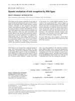
In Figure 1 we show a simplification of the FOCI network con-
structed by retaining the 4,000 strongest edges. We used this
edge-thresholding procedure to provide a comprehensible
two-dimensional visualization of the graph; all the results
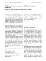
Simplification of the yeast FOCI coexpression network constructed by retaining the 4,000 strongest edges (= 1,729 vertices)Figure 1
Simplification of the yeast FOCI coexpression network constructed by retaining the 4,000 strongest edges (= 1,729 vertices). The colored vertices
represent a subset of the locally distinct subgraphs of the FOCI network; letters are as in Table 2, and further details can be found there. Some of the
locally distinct subgraphs of Table 2 are not represented in this figure because they involve subgraphs whose edge weights are not in the top 4,000 edges.
A
G
H
I
J
K
P
Q
R
S
U

T
N
O
L
M
B
D
F
E
C
R100.4 Genome Biology 2004, Volume 5, Issue 12, Article R100 Magwene and Kim />Genome Biology 2004, 5:R100
Table 1
Summary of queries for 38 metabolic pathways against the yeast FOCI coexpression network
Pathway Number of genes(in KEGG) Size of largest coherent subnetwork(s)
Carbohydrate metabolism
Glycolysis/gluconeogenesis 41 (47) 18*
Citrate cycle (TCA cycle) 27 (30) 18*
Pentose phosphate pathway 20 (27) 6*
Fructose and mannose metabolism 39 (46) 4
Galactose metabolism 25 (30) 8*
Ascorbate and aldarate metabolism 11 (13) 3
Pyruvate metabolism 32 (34) 8*
Glyoxylate and dicarboxylate metabolism 12 (14) 6*
Butanoate metabolism 27 (30) 7*
Energy metabolism
Oxidative phosphorylation 53 (76) 31*
ATP synthesis 21 (30) 7*
Nitrogen metabolism 24 (27) 3
Lipid metabolism
Fatty acid metabolism 13 (17) 3

Nucleotide metabolism
Purine metabolism 87 (99) 34*
Pyrimidine metabolism 72 (80) 15*
Nucleotide sugars metabolism 11 (14) 2
Amino acid metabolism
Glutamate metabolism 25 (27) 3
Alanine and aspartate metabolism 26 (27) 7*
Glycine, serine and threonine metabolism 36 (42) 7*
Methionine metabolism 13 (14) 6*
Valine, leucine and isoleucine biosynthesis 15 (16) 10*
Lysine biosynthesis 16 (20) 3
Lysine degradation 26 (30) 4
Arginine and proline metabolism 20 (24) 5*
Histidine metabolism 20 (25) 3
Tyrosine metabolism 27 (34) 2
Tryptophan metabolism 20 (25) 2
Phenylalanine, tyrosine and tryptophan
biosynthesis
21 (23) 6*
Metabolism of complex carbohydrates
Starch and sucrose metabolism 118 (139) 29
N-Glycans biosynthesis 43 (49) 13*
O-Glycans biosynthesis 18 (20) 2
Aminosugars metabolism 16 (20) 2
Keratan sulfate biosynthesis 18 (20) 2
Genome Biology 2004, Volume 5, Issue 12, Article R100 Magwene and Kim R100.5
comment reviews reports refereed researchdeposited research interactions information
Genome Biology 2004, 5:R100
discussed below were derived from analyses of the entire GCC of
the FOCI network.

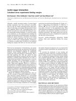
The mean, median and modal values for vertex degree in the
GCC are 4.87, 4 and 2 respectively. That is, each gene shows
significant expression relationships to approximately five
other genes on average, and the most common form of rela-
tionship is to two other genes. Most genes have five or fewer
neighbors, but there is a small number of genes (349) with
more than 10 neighbors in the FOCI network; the maximum
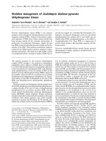
degree in the graph is 28 (Figure 2a). Thus, approximately 7%
of genes show significant expression relationships to a fairly
large number of other genes. The connectivity of the FOCI
network is not consistent with a power-law distribution (see
Additional data file 1 for a log-log plot of this distribution).
We estimated the distribution of path distances between pairs
of genes (defined as the smallest number of graph edges sep-
arating the pair) by randomly choosing 1,000 source vertices
in the GCC, and calculating the path distance from each
source vertex to every other gene in the network (Figure 2b).
The mean path distance is 6.46 steps, and the median is 6.0
(mode = 7). The maximum path distance is 16 steps. There-
fore, in the GCC of the FOCI network, random pairs of genes
are typically separated by six or seven edges.
Coherence of the FOCI network with known metabolic
pathways
To assess the biological relevance of our estimated coexpres-
sion network we compared the composition of 38 known met-
abolic pathways (Table 1) to our yeast coexpression FOCI
network. In a biologically informative network, genes that are
involved in the same pathway(s) should be represented as
coherent pieces of the larger graph. That is, under the
assumption that pathway interactions require co-regulation

and coexpression, the genes in a given pathway should be rel-
atively close to each other in the estimated global network.
We used a pathway query approach to examine 38 metabolic
pathways relative to our FOCI network. For each pathway, we
computed a quantity called the 'coherence value' that meas-
ures how well the pathway is recovered in a given network
model (see Materials and methods). Of the 38 pathways
Metabolism of complex lipids
Glycerolipid metabolism 56 (68) 12*
Inositol phosphate metabolism 87 (103) 10
Sphingophospholipid biosynthesis 101 (118) 11
Metabolism of cofactors and vitamins
Vitamin B6 metabolism 11 (14) 2
Folate biosynthesis 14 (17) 1
The values in the second column represent the number of pathway genes represented in the GCC of the yeast FOCI graph, with the total number of
genes assigned to the given pathway in parentheses. The third column indicates the number of pathway genes in the largest coherent subgraph
resulting from each pathway query. Pathways represented by coherent subgraphs that are significantly larger than are expected at random (p < 0.05)
are marked with asterisks.
Table 1 (Continued)
Summary of queries for 38 metabolic pathways against the yeast FOCI coexpression network
Topological properties of the yeast FOCI coexpression networkFigure 2
Topological properties of the yeast FOCI coexpression network.
Distribution of (a) vertex degrees and (b) path lengths for the network.
Vertex degree (k)
Path distance
Frequency
Frequency
0
1
12345678910111213141516

3 5 7 9 11 13 15 17 19 21 23 25 27
100
200
300
400
500
600
700
800
900
0
200,000
400,000
600,000
800,000
1,000,000
1,200,000
1,400,000
(a)
(b)
R100.6 Genome Biology 2004, Volume 5, Issue 12, Article R100 Magwene and Kim />Genome Biology 2004, 5:R100
tested, 19 have coherence values that are significant when
compared to the distribution of random pathways of the same
size (p < 0.05; see Materials and methods). Most of the path-
ways of carbohydrate and amino-acid metabolism that we
examined are coherently represented in the FOCI network. Of
each of the major categories of metabolic pathways listed in
Table 1, only lipid metabolism and metabolism of cofactors
and vitamins are not well represented in the FOCI network.
The five largest coherent pathways are glycolysis/gluconeo-

genesis, the TCA cycle, oxidative phosphorylation, purine
metabolism and synthesis of N-glycans. Other pathways that
are distinctive in our analysis include the glyoxylate cycle (6
of 12 genes in largest coherent subnetwork), valine, leucine,
and isoleucine biosynthesis (10 of 15 genes), methionine
metabolism (6 of 13 genes), phenylalanine, tyrosine, and
tryptophan metabolism (two subnetworks each of 6 genes).
Several coherent subsets of the FOCI network generated by
these pathway queries are illustrated in the Additional data
file 1.
Combined analysis of core carbohydrate metabolism
In addition to being consistent with individual pathways, a
useful network model should capture interactions between
pathways. To explore this issue we queried the FOCI network
on combined pathways and again measured its coherence. We
illustrate one such combined query based on four related
pathways involved in carbohydrate metabolism: glycolysis/
gluconeogenesis, pyruvate metabolism, the TCA cycle and the
glyoxylate cycle.
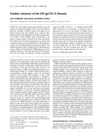
Figure 3 illustrates the largest subgraph extracted in this
combined analysis. The combined query results in a subset of
the FOCI network that is larger than the sum of the subgraphs
estimated separately from individual pathways because it also
admits non-query genes that are connected to multiple path-
ways. The nodes of the graph are colored according to their
membership in each of the four pathways as defined by the
Kyoto Encyclopedia of Genes and Genomes (KEGG). Many
gene products are assigned to multiple pathways. This is par-
ticularly evident with respect to the glyoxylate cycle; the only
genes uniquely assigned to this pathway are ICL1 (encoding

an isocitrate lyase) and ICL2 (a 2-methylisocitrate lyase).
In this combined pathway query the TCA cycle, glycolysis/
gluconeogenesis, and glyxoylate cycle are each represented
primarily by a single two-step connected subgraph (see Mate-
rials and methods). Pyruvate metabolism on the other hand,
is represented by at least two distinct subgraphs, one includ-
ing {PCK1, DAL7, MDH2, MLS1, ACS1, ACH1, LPD1, MDH1}
and the other including {GLO1, GLO2, DLD1, CYB2}. This
second set of genes encodes enzymes that participate in a
branch of the pyruvate metabolism pathway that leads to the
degradation of methylglyoxal (methylglyoxal → L-lactalde-
hyde → L-lactate → pyruvate and methylglyoxal → (R)-S-lac-
toyl-glutathione → D-lactaldehyde → D-lactate → pyruvate)
[12,13]. In the branch of methylglyoxal metabolism that
involves S-lactoyl-glutathione, methyglyoxal is condensed
with glutathione [12]. Interestingly, two neighboring non-
query genes, GRX1 (a neighbor of GLO2) and TTR1 (neighbor
of CYB2), encode proteins with glutathione transferase
activity.
The position of FBP1 in the combined query is also interest-
ing. The product of FBP1 is fructose-1,6-bisphosphatase, an
enzyme that catalyzes the conversion of beta-d-fructose 1,6-
bisphosphate to beta-D-fructose 6-phosphate, a reaction
associated with glycolysis. However, in our network it is most
closely associated with genes assigned to pyruvate metabo-
lism and the glyoxylate cycle. The neighbors of FBP1 in this
query include ICL1, MLS1, SFC1, PCK1 and IDP3. With the
exception of IDP3, the promoters of all of these genes (includ-
ing FBP1) have at least one upstream activation sequence that
can be classified as a carbon source-response element

(CSRE), and that responds to the transcriptional activator
Cat8p [14]. This set of genes is expressed under non-fermen-
tative growth conditions in the absence of glucose, conditions
characteristic of the diauxic shift [15]. Considering other
genes in the vicinity of FBP1 in the combined pathway query
we find that ACS1, IDP2, SIP4, MDH2, ACH1 and YJL045w
have all been shown to have either CSRE-like activation
sequences and/or to be at least partially Cat8p dependent
[14]. The association among these Cat8p-activated genes per-
sists when we estimate the FOCI network without including
the data of DeRisi et al. [15], suggesting that this set of inter-
actions is not merely a consequence of the inclusion of data
collected from cultures undergoing diauxic shift.
The inclusion of a number of other genes in the carbohydrate
metabolism subnetwork is consistent with independent evi-
dence from the literature. For example, McCammon et al.
[16] identified YER053c as among the set of genes whose
expression levels changed in TCA cycle mutants.
Although many of the associations among groups of genes
revealed in these subgraphs can be interpreted either in terms
of the query pathways used to construct them or with respect
to related pathways, a number of association have no obvious
biological interpretation. For example, the tail on the left of
the graph in Figure 3, composed of LSC1, PTR2, PAD1, OPT2,
ARO10 and PSP1 has no clear known relationship.
Locally distinct subgraphs
The analysis of metabolic pathways described above provides
a test of the extent to which known pathways are represented
in the FOCI graph. That is, we assumed some prior knowledge
about network structure of subsets of genes and asked

whether our estimated network is coherent vis-à-vis this
prior knowledge. Conversely, one might want to find interest-
ing and distinct subgraphs within the FOCI network without
the injection of any prior knowledge and ask whether such
subgraphs correspond to particular biological processes or
Genome Biology 2004, Volume 5, Issue 12, Article R100 Magwene and Kim R100.7
comment reviews reports refereed researchdeposited research interactions information
Genome Biology 2004, 5:R100
functions. To address this second issue we developed an algo-
rithm to compute 'locally distinct subgraphs' of the yeast
FOCI coexpression network as detailed in the Materials and
methods section. Briefly, this is an unsupervised graph-
search algorithm that defines 'interestingness' in terms of
local edge topology and the distribution of local edge weights
on the graph. The goal of this algorithm is to find connected
subgraphs whose edge-weight distribution is distinct from
that of the edges that surround the subgraph; thus, these
locally distinct subgraphs can be thought of as those vertices
and associated edges that 'stand out' from the background of
the larger graph as a whole.
We constrained the size of the subgraphs to be between seven
and 150 genes, and used squared marginal correlation coeffi-
cients as the weighting function on the edges of the FOCI
graph. We found 32 locally distinct subgraphs, containing a
total of 830 genes (Table 2). Twenty-four out of the 32 sub-
graphs have consistent Gene Ontology (GO) annotation terms
[17] with p-values less than 10
-5
(see Materials and methods).
This indicates that most locally distinct subgraphs are highly

enriched with respect to genes involved in particular biologi-
cal processes or functions. Members of the 21 largest locally
distinct subgraphs are highlighted in Figure 1. The complete
list of subgraphs and the genes assigned to them is given in
Additional data file 2.
The five largest locally distinct subgraphs have the following
primary GO annotations: protein biosynthesis (subgraphs A
and B); ribosome biogenesis and assembly (subgraph C);
response to stress and carbohydrate metabolism (subgraph
K); and sporulation (subgraph N). Several of these subgraphs
show very high specificity for genes with particular GO anno-
tations. For example, in subgraphs A and B approximately
97% (32 out of 33) and 95.5% (64 out of 67) of the genes are
assigned the GO term 'protein biosynthesis'.
Largest connected subgraph resulting from combined query on four pathways involved in carbohydrate metabolism: glycolysis/gluconeogenesis (red); pyruvate metabolism (yellow); TCA cycle (green); and the glyoxylate cycle (pink)Figure 3
Largest connected subgraph resulting from combined query on four pathways involved in carbohydrate metabolism: glycolysis/gluconeogenesis (red);
pyruvate metabolism (yellow); TCA cycle (green); and the glyoxylate cycle (pink). Genes encoding proteins involved in more than one pathway are
highlighted with multiple colors. Uncolored vertices represent non-pathway genes that were recovered in the combined pathway query. See text for
further details.
ACS1
ACH1
IST2
PGI1
GRX1
GLK1
YCP4
CIT2
ADP1
PGK1
GPM2

IDP1
DLD1
TPI1
KGD2
HSP42
SDH4
COX20
GLO2
ARO10
PSP1
TTR1
PAD1
YER053C
ICL1
LPD1
ACT1
YFL054C
PYC1
HXK2
MSP1
TDH3
ADE3
PFK1
YGR243W
LSC2
ENO1
ENO2
KGD1
OM45
DAL7

YJL045W
TDH1
SIP4
TDH2
SFC1
ATP2
FBA1
MDH1
SDH1
MCR1
GPM1
YKL187C
PTR2
PCK1
SDH2
PDC1
PDC5
ACS2
IDP2
TFS1
ECM38
ACO1
TAL1
ADE13
FBP1
GLO1
TSA1
GSF2
CYB2
NDI1

ERG13
FET3
ADH3
PGM2
YMR110C
NDE1
ALD2
GAD1
YMR323W
IDP3
NCE103
IDH1
LEU4
MLS1
ATG3
ADH1
MDH2
GLO4
IDH2
LSC1
YOR215C
YOR285W
PYK2
MRS6
ALD4
ERG10
ODC1
FUM1
ICL2
OPT2

TCA
cycle
Glycolysis/
gluconeogenesis
Pyruvate
metabolism
Glyoxylate
cycle
Acetyl-CoA
Pyruvate
Acetaldehyde
Acetate
R100.8 Genome Biology 2004, Volume 5, Issue 12, Article R100 Magwene and Kim />Genome Biology 2004, 5:R100
Subgraph P is also relatively large and contains many genes
with roles in DNA replication and repair. Similarly, 21 of the
34 annotated genes in Subgraph F have a role in protein
catabolism. Three medium-sized subgraphs (S, T, U) are
strongly associated with the mitotic cell cycle and cytokinesis.
Other examples of subgraphs with very clear biological roles
are subgraph R (histones) and subgraph Z (genes involved in
conjugation and sexual reproduction). Subgraph X contains
genes with roles in methionine metabolism or transport.
Some locally distinct subgraphs can be further decomposed.
For example, subgraph K contains at least two subgroups.
One of these is composed primarily of genes encoding chap-
erone proteins: STI1, SIS1, HSC82, HSP82, AHA1, SSA1,
Table 2
Summary of locally distinct subgraphs of the yeast FOCI coexpression network
Subgraph Number of genes Number unkown Major GO terms p-value
A 33 0 Protein biosynthesis (32) 1.82e-30

B 67 2 Protein biosynthesis (64) 2.20e-61
C 124 26 Ribosome biogenesis and assembly (74) 2.10e-89
D 10 0 Glycolysis/gluconeogenesis (8) 6.29e-20
E 7 1 Carboxylic/organic acid metabolism (4) 5.07e-05
F 41 7 Ubiquitin dependent protein catabolism (21) 1.37e-31
G 14 4 Cell organization and biogenesis (7) 1.60e-04
H 7 0 Main pathways of carbohydrate metabolism (4) 2.46e-07
I 13 0 Electron transport (7) 2.00e-15
J 13 0 Glutamate biosynthesis/TCA cycle (4) 7.09e-10
K 71 25 Response to stress (17); carbohydrate metabolism (13) 3.94e-11
L 10 4 Response to stress (2) 3.35e-02
N 149 51 Sporulation (27) 2.23e-29
M 5 2 Mitochondrial matrix (5); mitochondrial ribosome (4) 2.83e-09
O 7 2 Meiosis (4) 3.77e-07
P 52 13 Cell proliferation (32); DNA replication and chromosome cycle
(28)
1.12e-28
Q 26 21 Telomerase-independent telomere maintenance (5) 1.82e-14
R 7 0 Chromatin assembly/disassembly (7) 4.25e-18
S 14 5 Cell wall (4); bud (4) 4.47e-05
T 24 8 Cell proliferation (15); mitotic cell cycle (9) 6.54e-16
U 21 4 Cell separation during cytokinesis (4); cell proliferation (9); cell
wall organization and biogenesis (5)
5.27e-10
V 12 4 Metabolism (7) 2.48e-02
W 10 9 Nine of ten are members of the seripauperin gene family NA
X 9 0 Sulfur amino acid metabolism (6); amino acid metabolism (3) 3.33e-13
Y 7 1 Cell growth and maintenance (6) 7.50e-04
Z 19 2 Conjugation with cellular fusion (13) 1.82e-21
AA 8 4 Biotin biosynthesis (2) 1.81e-06

BB 7 0 Response to abiotic stimulus (2) 1.48e-02
CC 9 5 Six of nine members belong to COS family of subtelomerically
encoded proteins
NA
DD 18 7 Cell growth and/or maintenance (8) 4.43e-03
EE 11 3 Vitamin B6 metabolism (2) 2.58e-05
FF 7 0 Ty element transposition (7) 6.01e-14
The columns of the table summarize the total size of the locally distinct subgraph, the number of genes in the subgraph that are unannotated
(according to the GO Slim annotation from the Saccharomyces Genome Database of December 2003), the primary GO term(s) associated with the
subgraph, and a p-value indicating the frequency at which one would expect to find the same number of genes assigned to the given GO term in a
random assemblage of the same size.
Genome Biology 2004, Volume 5, Issue 12, Article R100 Magwene and Kim R100.9
comment reviews reports refereed researchdeposited research interactions information
Genome Biology 2004, 5:R100
SSA2, SSA4, KAR2, YPR158w, YLR247c. The other group
contains genes primarily involved in carbohydrate metabo-
lism. These two subgroups are connected to each other exclu-
sively through HSP42 and HSP104.
Three of the locally distinct subgraphs - Q, W and CC - are
composed primarily of genes for which there are no GO bio-
logical process annotations. Interestingly, the majority of
genes assigned to these three groups are found in subtelom-
eric regions. These three subgraphs are not themselves
directly connected in the FOCI graph, so their regulation is
not likely to be simply an instance of a regulation of subtelo-
meric silencing [18]. Subgraph Q includes 26 genes, five of
which (YRF1-2, YRF1-3, YRF1-4, YRF1-5, YRF1-6)
correspond to ORFs encoding copies of Y'-helicase protein 1
[19]. Eight additional genes (YBL113c, YEL077c, YHL050c,
YIL177c, YJL225c, YLL066c, YLL067c, YPR204w) assigned

to this subgraph also encode helicases. This helicase sub-
graph is closely associated with subgraph P, which contains
numerous genes involved in DNA replication and repair (see
Figure 1). Subgraph W contains 10 genes, only one of which is
assigned a GO process, function or component term. How-
ever, nine of the 10 genes in the subgraph (PAU1, PAU2,
PAU4, PAU5, PAU6, YGR294w, YLR046c, YIR041w,
YLL064c) are members of the seripauperin gene family [20],
which are primarily found subtelomerically and which encode
cell-wall mannoproteins and may play a role in maintaining
cell-wall integrity [18]. Another example of a subgraph corre-
sponding to a multigene family is subgraph CC, which
includes nine subtelomeric ORFs, six of which encode
proteins of the COS family. Cos proteins are associated with
the nuclear membrane and/or the endoplasmic reticulum
and have been implicated in the unfolded protein response
[21].
As a final example, we consider subgraph FF, which is com-
posed of seven ORFs (YAR010c, YBL005w-A, YJR026w,
YJR028w, YML040w, YMR046c, YMR051c) all of which are
parts of Ty elements, encoding structural components of the
retrotransposon machinery [22,23]. This set of genes nicely
illustrates the fact that delineating locally distinct groups can
lead to the discovery of many interesting interactions. There
are only six edges among these seven genes in the estimated
FOCI graph, and the marginal correlations among the
correlation measures of these genes are relatively weak (mean
r ~ 0.62). Despite this, the local distribution of edge weights
in FOCI graph is such that this group is highlighted as a sub-
graph of interest. Locally strong subgraphs such as these can

also be used as the starting point for further graph search pro-
cedures. For example, querying the FOCI network for imme-
diate neighbors of the genes in subgraph FF yields three
additional ORFs - YBL101w-A, YBR012w-B, and RAD10.
Both YBL101w-A and YBR012w-B are Ty elements, whereas
RAD10 encodes an exonuclease with a role in recombination.
Discussion
Comparisons with other methods
Comparing the performance of different methods for analyz-
ing gene-expression data is a difficult task because there is
currently no 'gold standard' to which an investigator can turn
to judge the correctness of a particular result. This is further
complicated by the fact that different methods employ dis-
tinct representations such as trees, graphs or partitions that
cannot be simply compared. With these difficulties in mind,
we contrast and compare our FOCI method to three popular
approaches for gene expression analysis - hierarchical clus-
tering [1], Bayesian network analysis [10] and relevance net-
works [7,24,25]. Like the FOCI networks described in this
report, both Bayesian networks and relevance networks rep-
resent interactions in the form of network models, and can, in
principle, capture complex patterns of interaction among var-
iables in the analysis. Relevance networks also share the
advantage with FOCI networks that, depending on the scor-
ing function used, they can be estimated efficiently for very
large datasets.
Comparison with relevance networks
Relevance networks are graphs defined by considering one or
more scoring functions and a threshold level for every pair of
variables of interest. Pairwise scores that rise above the

threshold value are considered significant and are repre-
sented by edges in the graph; interactions below this thresh-
old are discarded [25]. As applied to gene-expression
microarray data, the scoring functions used most typically
have been mutual information [7] or a measure based on a
modified squared sample correlation coefficient
[24]).
We estimated a relevance network for the same 5007-gene
dataset used to construct the FOCI network. The scoring
function employed was with a threshold value of ± 0.5.
The resulting relevance network has 13,049 edges and a GCC
with 1,543 vertices and 12,907 edges. The next largest con-
nected subgraph of the relevance network has seven vertices
and seven edges. There are a very large number of connected
subgraphs (3,341) that are composed of pairs or singletons of
genes.
To compare the performance of the relevance network with
the FOCI network we used the pathway query approach
described above to test the coherence of the 38 metabolic
pathways described previously. Of the 38 metabolic pathways
tested, nine have significant coherence values in the relevance
network. These coherent pathways include: glycolysis/gluco-
neogenesis, the TCA cycle, oxidative phosphorylation, ATP
synthesis, purine metabolism, pyrimidine metabolism,
methionine metabolism, amino sugar metabolism, starch and
sucrose metabolism. Two of these pathways - amino sugar
metabolism and starch and sucrose metabolism - are not sig-
nificantly coherent in the FOCI network. However, there are
(
ˆ

(/rr rr
22
= abs( ))
ˆ
r
2
R100.10 Genome Biology 2004, Volume 5, Issue 12, Article R100 Magwene and Kim />Genome Biology 2004, 5:R100
12 metabolic pathways that are coherent in the FOCI network
but not coherent in the relevance network. On balance, the
FOCI network model provides a better estimator of known
metabolic pathways than does the relevance network
approach.
Comparison with hierarchical clustering and Bayesian
networks
To provide a common basis for comparison with hierarchical
clustering and Bayesian networks, we explored the dataset of
Spellman et al. [26] which includes 800 yeast genes meas-
ured under six distinct experimental conditions (a total of 77
microarrays; this data is a subset of the larger analysis
described in this paper). Spellman et al. [26] analyzed this
dataset using hierarchical clustering. Friedman et al. [10]
used their 'sparse candidate' algorithm to estimate a Bayesian
network for the same data, treating the expression measure-
ments as discrete values. For comparison with Bayesian net-
work analysis we referenced the interactions highlighted in
the paper by Friedman et al. and the website that accompa-
nies their report [27]. For the purposes of the FOCI analysis
we reduced the 800 gene dataset to 741 genes for which there
were no more than 10 missing values. We conducted a FOCI
analysis on these data using a partial correlation threshold of

0.33. The resulting FOCI network had 1599 edges and a GCC
of 700 genes (the 41 other genes are represented by sub-
graphs of gene pairs or singletons).
On the basis of hierarchical clustering analysis of the 800 cell-
cycle-regulated genes, Spellman et al. [26] highlighted eight
distinct coexpressed clusters of genes. They showed that most
genes in the clusters they identified share common promoter
elements, bolstering the case that these clusters indeed corre-
spond to co-regulated sets of genes (see [26] for description
and discussion of these clusters).
Applying our algorithm for finding locally distinct subgraphs
to the FOCI graph based on these same data (with size con-
straints min = 7, max = 75) we found 10 locally distinct sub-
graphs. Seven of these subgraphs correspond to major
clusters in the hierarchical cluster analysis (the MCM cluster
of Spellman et al. [26] is not a locally distinct subgraph). At
this global level both FOCI analysis and hierarchical cluster-
ing give similar results. While the coarse global structure of
the FOCI and hierarchical clustering are similar, at the inter-
mediate and local levels the FOCI analysis reveals additional
biologically meaningful interactions that are not represented
in the clustering analysis. An example of interactions at an
intermediate scale involves the clusters referred to as Y' and
CLN2 in Spellman et al. [26] Genes of the CLN2 cluster are
involved primarily in DNA replication. The Y' cluster contains
genes known to have DNA helicase activity. The topology of
the FOCI network indicates that these are relatively distinct
subgraphs, but also highlights a number of weak-to-moderate
statistical interactions between the Y' and CLN2 genes (and
almost no interactions between the Y' genes and any other

cluster). Thus the FOCI network estimate provides inference
of more subtle functional relationships that cannot be
obtained from the clustering family of methods.
An example at a more local scale involves the MAT cluster of
Spellman et al. [26] This cluster includes a core set of genes
whose products are known to be involved in conjugation and
sexual reproduction. In the FOCI network one of the locally
distinct subgraphs is almost identical to the MAT cluster, and
includes KAR4, STE3, LIF1, FUS1, SST2, AGA1, SAG1, MF
α
2
and YKL177W (MF
α
1 is not included in the FOCI analysis
because there were more than 10 missing values). The FOCI
analysis additionally shows that this set of genes is linked to
another subgraphs that includes AGA2, STE2, MFA1, MFA2
and GFA3. This second set of genes are also involved in con-
jugation, sexual reproduction, and pheromone response.
AGA1 and AGA2 form the bridge between these two sub-
graphs (the proteins encoded by these two genes, Aga1p and
Aga2p, are subunits of the cell wall glycoprotein
α
-agglutinin
[28]). These two sets of genes therefore form a continuous
subnetwork in the FOCI analysis, whereas the same genes are
dispersed among at least three subclusters in the hierarchical
clustering. We interpret the difference as resulting from the
fact that the FOCI network can include relatively weak inter-
actions among variables, as long as the variables are not first

order conditionally independent. For example, the marginal
correlation between AGA1 and AGA2 is only 0.63, between
AGA1 and GFA1 is 0.59, and between AGA2 and MFA1 only
0.61. Hierarchical clustering or other analyses based solely on
marginal correlations will typically fail to highlight such rela-
tively weak interactions among genes.
Because hierarchical clustering constrains relationships to
take the form of strict partitions or nested partitions, this type
of analysis seems best suited to highlight the overall coarse
structure of co-regulatory relationships. The FOCI method,
because it admits a more complex set of topological relation-
ships, is well suited to capturing both global and local struc-
ture of transcriptional interactions.
Graphical models, like the FOCI method, exploit conditional
independence relationships to derive a model that can be rep-
resented using a graph or network structure. Unlike the FOCI
model, general graphical models represent a complete factor-
ization of a multivariate distribution. In the case of Bayesian
networks it is also possible to assign directionality to the
edges of the network model. However, these advantages come
at the cost of complexity - Bayesian networks are costly to
compute - and generally this complexity scales exponentially
with the number of vertices (genes). The estimation of a FOCI
network is computationally much less complex than the esti-
mation of a Bayesian network. Both methods allow for a
richer set of potential interactions among genes than does
hierarchical clustering. We therefore expect that both meth-
ods should be able to highlight biologically interesting inter-
actions, at both local and global scales. Friedman et al. [10]
Genome Biology 2004, Volume 5, Issue 12, Article R100 Magwene and Kim R100.11

comment reviews reports refereed researchdeposited research interactions information
Genome Biology 2004, 5:R100
analyzed the 800-gene dataset of Spellman et al. [26] and
highlighted a number of relationships that are assigned high
confidence in their analysis. Relationships that were recov-
ered under both a multinomial and Gaussian model include
STE2-MFA2, CTS1-DSE2(YHR143w), OLE1-FAA4, KIP3-
MSB1, SHM2-GCV2, DIP5-ARO9 and SRO4-YOL007c. All of
these relationships, with the exception of SRO5-YOL007c, are
present in the FOCI analysis of the same data.
Comparisons of the local topology of each network, based on
examining the edge relationships for a number of query
genes, suggests that the FOCI and Bayesian networks are
broadly similar. There are of course, examples of biologically
interpretable interactions that are present in the FOCI analy-
sis but not in the Bayesian network and vice versa. For exam-
ple, using a multinomial model, Friedman et al.
demonstrated an interaction between ASH1 and FAR1, both
of which are known to participate in the mating type switch in
yeast. This relationship is absent in the FOCI network. Simi-
larly, the relationship between AGA1 and AGA2 that is
highlighted in the FOCI analysis does not appear in the multi-
nomial Bayesian network analysis.
Review of FOCI assumptions
As with all analytical tools, careful consideration of the
assumptions underlying the FOCI network method is neces-
sary to understand the limits of the inferences one can draw.
For example, our current framework limits consideration to
linear relationships as measured by correlations and partial
correlations. These assumptions may be relaxed, allowing for

other types of distributions and relationships among varia-
bles (for example, monotone and curvilinear relationships),
but there is an inevitable trade-off to be made in terms of
computational complexity and statistical power. However, as
seen in our analysis, many biologically interesting relation-
ships among gene expression measures appear to be approx-
imately linear. Biologically speaking, it is important to keep in
mind that the graphs resulting from a FOCI analysis of gene-
expression measurements should properly be considered
coexpression or co-regulation networks and not genetic regu-
latory networks per se. While the clusters and patterns of
coexpression summarized by the FOCI network may result
from particular regulatory dynamics, no causal hypothesis of
regulatory interaction is implied by the network.
Conclusions
Biology demands that the analytical tools we use for func-
tional genomics should be able to capture and represent com-
plex interactions; practical considerations stemming from the
magnitude and scope of genomic data require the use of tech-
niques that are computable and relatively efficient. The FOCI
framework we have used for representing genomic coexpres-
sion patterns in terms of a weighted graph satisfies both these
constraints. FOCI networks are readily computable, even for
very large datasets. Comparisons with known metabolic path-
ways show that many key biological interactions are captured
by FOCI networks, and the algorithm we provide for finding
locally distinct subgraphs provides a mechanism for discover-
ing novel associations based on local graph topology. The
subgraphs and patterns of interactions that we are able to
demonstrate based on such analyses are strongly consistent

with known biological processes and functions, indicating
that the FOCI network method is a powerful tool for summa-
rizing biologically meaningful coexpression patterns. Fur-
thermore, the kinds of interactions captured by network
analysis are typically more natural than the clustering family
of analyses where biased and unstable results can be forced by
the algorithm. Secondary analysis based on the network
properties also reveal additional subtle structure. For exam-
ple, our procedure for finding locally distinct subgraphs
reveals associated genes whose pairwise interactions may be
globally weak but relatively strong compared to their local
interactions. While the results reported here focus on the
analysis of gene expression measurements, the FOCI
approach can be applied to any type of quantitative data mak-
ing it a generally suitable technique for exploratory analyses
of functional genomic data.
Materials and methods
A statistical/geometrical model for estimating
coexpression networks
The approach we employ to estimate coexpression networks
is based on a general statistical technique we have developed
for representing the associations among a large number of
variables in terms of a weighted, undirected graph. The tech-
nique is based on the consideration of so-called 'first-order'
conditional independence relationships among variables,
hence we call the graphs that result from such analyses first-
order conditional independence, FOCI, networks. The net-
work representation that results from a FOCI analysis also
has a dual geometrical interpretation in terms of proximity
relationships defined with respect to the geometry of correla-

tions and partial correlations. We outline the statistical and
geometrical motivations underlying our approach below.
First-order conditional independence networks
A FOCI network is a graph, G = {V,E}, where the vertex set, V,
represents the variables of interest and the edge set, E, repre-
sents interactions among the variables. e
ij
is an edge in G, if
and only if there is no other variable in the analysis, k(k ≠ k ≠
k) such that or , where
is a modified partial correlation between i and j condi-
tioned on k. takes values in the range -1 ≤ ≤ 1.
is approximately zero when i and j are independent condi-
ˆ
.
r
ij k
≈ 0
ˆ
.
r
ij k
< 0
ˆ
||| || |
.
r
rrr
rr
ij k

ij ik jk
ik jk
=
−
−−
()
11
1
22
ˆ
.
r
ij k
ˆ
.
r
ij k
ˆ
.
r
ij k
ˆ
.
r
ij k
R100.12 Genome Biology 2004, Volume 5, Issue 12, Article R100 Magwene and Kim />Genome Biology 2004, 5:R100
tional on k. is positive when the marginal correlation,
ρ
ij
, and the standard partial correlation,

ρ
ij.k
, agree in sign,
and is negative otherwise. Cases where the marginal and con-
ditional correlations are of opposite sign are examples of
'Simpson's paradox', which usually indicates that there is a
lurking or confounding effect of the conditioning variable (see
[29] for a general discussion of such relationships).
While true biological interactions may sometimes lead to
inverted conditional associations, their interpretation can be
complicated; therefore in the analysis presented above, we
did not connect edges when the relationships became
inverted. However, one can also keep such edges for subse-
quent analysis if there is reasonable functional justification.
When such sign-reversed edges are ignored, we will call this
the sign-restricted FOCI network. This definition means that
variables i and j are connected in the FOCI network if there is
no other variable in the analysis for which i and j are condi-
tionally independent or which causes an association reversal.
Because we restrict the conditioning set to single variables,
these are so called 'first-order' conditional interactions (mar-
ginal correlations correspond to zero-order conditional inter-
actions; partial correlations given two conditioning variables
are second-order conditional interactions, etc). If i and j are
conditionally independent given k we write this as (i ⊥ j|k).
Using an information theoretic interpretation suggested by
Lauritzen [9], the statement (i ⊥ j|k) implies that if we observe
the variable k, there is no additional information about i that
we gain by also observing j (and vice versa). Because the edges
of the FOCI network indicate pairs of variables that are not

conditionally independent, one can interpret the FOCI graph
as a summary of all the pairwise interactions that can not be
'explained away' by any other single variable in the analysis.
Unlike standard graphical models, a FOCI network does not
represent a factorization of a multivariate distribution into
the product of simpler distributions. However, below we
show that a sign-restricted FOCI graph has a unique geomet-
ric interpretation in terms of proximity relationships in the
multidimensional space that represents the correlations
among variables. This geometric interpretation suggests that
the FOCI model should be a generally useful approach for
exploratory analyses of very high-dimensional datasets.
Our FOCI approach is similar to a framework developed by de
Campos and Huete [30] for estimating belief networks. These
authors developed an algorithm based on the application of
zero- and first-order conditional independence test to learn
the 'prior skeleton' of a Bayesian network, followed by a
refinement procedure that uses higher-order interactions
sparingly.
Geometrical model of first-order conditional
independence
Above we described the FOCI network model in statistical
terms. Here we provide a geometrical interpretation of FOCI
graphs. We show that a FOCI network is equivalent to a prox-
imity graph of the variables of interest (genes in the current
analysis). More specifically, we demonstrate that a sign-
restricted FOCI network is a 'Gabriel graph' in the geometric
space that represents the relationships among the variables.
A Gabriel graph, introduced by Gabriel and Sokal [31], is a
type of proximity graph. Let B(x,r) denote an open n-sphere

centered at the point x with radius r, and let d(p,q) denote the
Euclidean distance function. Given a set of points, P = {p
1
p
2
,
, p
n
}, in an n-dimensional Euclidean space, (p
i
, p
j
) is an edge
in the Gabriel graph if no other point, p
k
(i ≠ k, j ≠ k) in P falls
within the diameter sphere defined by B((p
i
= p
j
)/2, d(p
i
, p
j
)/
2). That is, p
i
and p
j
are connected in the Gabriel graph if no

other point falls within the sphere that has the chord p
i
, p
j
as
its diameter [32].
Geometry of marginal and partial correlations and
conditional independence
One can represent random variables as vectors in the space of
the observations (often called object space or subject space
[33,34]). In such a representation, a set of mean centered and
standardized variables correspond to unit vectors whose
heads lie on the surface of an n-dimensional hypersphere
(where n is the number of observations). In this representa-
tion, the correlation between two random variables, x and y,
is given by the cosine of the angle between their vectors. We
will refer to this construction as the 'correlational hyper-
sphere'. The partial correlation between x and y given z is
equivalent to the cosine of the angle between the residual vec-
tors obtained by projecting x and y onto z. The vectors x, y and
z form the vertices, A, B, and C, of a spherical triangle on that
hypersphere with associated angles
γ
,
λ
, and
φ
. Then,
ρ
xy.z

=
cos(
φ
),
ρ
xz.y
= cos(
λ
), and
ρ
yz.x
= cos(
γ
) [35]. Given this geo-
metric construction of partial correlations in terms of spheri-
cal triangles, conditional independence, defined as
ρ
xy.z
= 0
for the multivariate normal, is obtained when cos(
φ
) = 0 (that
is, when the
φ
=
π
/2). The set of z vectors that satisfy this con-
dition defines a circle (actually a hypersphere of dimension n
- 1) on the hypersphere whose diameter is the spherical chord
between x and y. If the projection of z onto the hypersphere

lies outside of this circle then
ρ
xy.z
is positive, inside the circle
ρ
xy.z
is negative (with
ρ
xy.z
= -1 along the chord between x and
y).
The sign-restricted FOCI network construction corresponds
to the graph obtained by connecting variables i and j only if no
third variable falls within the diameter sphere defined by i
and j on the correlational hypersphere, or by the diameter
sphere defined by i and -j when r
ij
< 0 (allowing for deviations
due to sampling). This is the same criteria of proximity that
defines a Gabriel graph. A FOCI graph is therefore a summary
ˆ
.
r
ij k
Genome Biology 2004, Volume 5, Issue 12, Article R100 Magwene and Kim R100.13
comment reviews reports refereed researchdeposited research interactions information
Genome Biology 2004, 5:R100
of relative proximity relationships among the variables of
interest, defined with respect to the geometry of correlations
when restricted to the cases when the partial correlation signs

are consistent with the marginal correlations.
FOCI network algorithm
A simple algorithm for estimating a network based on first-
order conditional independence relationships is described
below. The results of this algorithm can be represented as a
graph where the vertices represent the variables of interest
(genes) and the edges represent interactions among variables
that show at least first-order conditional dependence. A
library of functions for estimating FOCI networks, imple-
mented in the Python programming language, is available
from the authors on request.
We use vanishing partial correlations [8,36] to test whether
pairs of genes are conditionally independent given any other
single variable in the analysis. Strictly speaking, if the data are
not multivariate normal, then zero partial correlations need
not imply conditional independence, but rather conditional
uncorrelatedness [37]. However, regardless of distributional
assumptions, zero partial correlations among variates are of
interest as long as the relationship between the variables has
a strong linear component [38].
FOCI algorithm
1. Estimate marginal associations. For a set of p varia-
bles, indexed by i and j, calculate the p × p correlation matrix,
C, where C
i,j
= corr(i, j) for all i, j; i = 1 p, j = 1 p.
2. Construct saturated graph. Construct a p × p adja-
cency matrix, G. Let G
i,j
= 1 for all i, j.

3. Prune zero-order independent edges. For each pair
of variables, (i, j), if C
i,j
<T
crit
(or some appropriately chosen
function, f(C
i,j
) <T
crit
), where T
crit
is a threshold value for
determining marginal/conditional independence (see
below), then set G
i,j
= 0. G defines a marginal independence
graph.
4. Estimate first-order relationships. For each pair of
variables (i, j) in G calculate , the minimum partial cor-
relation between i and j, conditioned on each of the other var-
iables in the analysis taken one at a time.
for all k such that i ≠ k and j ≠ k and (i, k) and (j, k) are both
edges in G. is the sample modified partial correlation
coefficient as defined in equation (1).
5. Prune first-order independent edges. If <T
crit
(or f() <T
crit
then set G

i,j
= 0.
The resulting adjacency matrix G, can be represented as an
undirected graph, with p vertices, whose edge set is defined
by the non-zero elements in G. The edges of this graph can be
represented as either unweighted (all edges having equal
weight) or with weights defined by some function of corr(i, j)
or . If we assume multivariate normality we can use
Fisher's z-transformation [39] to normalize the expected dis-
tribution of correlation/partial correlations and use standard
tables of the normal distribution to define T
crit
for a given
edge-wise false-positive rate. Alternatively, one can define
T
crit
by other methods such as via permutation analysis to
define a null distribution for . While the FOCI approach
requires that one define a critical threshold for determining
conditional independence, this threshold is in theory a func-
tion of the sample size and the null distribution of
rather than the somewhat fuzzier distinction between 'strong'
and 'weak' correlation that most pairwise network estimation
approaches require.
Estimating the yeast FOCI coexpression network
We used the FOCI network algorithm to estimate a coexpres-
sion network for the budding yeast, Saccharomyces cere-
visae. The data used in our analysis are drawn from publicly
available microarray measurements of gene expression
described in DeRisi et al. [15], Chu et al. [40] and Spellman et

al. [26]. These data represent relative measurements of gene
expression taken at different points in the cell cycle in yeast
cultures synchronized using a variety of different mecha-
nisms [26] or in the context of specific physiological process
such as diauxic shift [15] or sporulation [40]. The data were
log
2
-transformed, duplicate and missing data were removed
and any ORFs listed as 'dubious' in the Saccharomyces
Genome Database as of December 2003 were filtered out. The
final dataset consisted of expression measurements for 5,007
ORFs represented by 87 microarrays (see Rifkin et al. [41] for
a full description of the pretreatment of these data). The mean
centered data were treated as continuous variables for the
purposes of our analysis.
Microarray measurements, especially spotted microarrays,
are subject to a variety of systematic effects such as those due
to dye biases and print-tip effects, and a number of methods
have been devised to normalize and correct for such biases
[42,43]. However, the data analyzed here include both spot-
ted DNA microarray measurements and expression measure-
ments based on Affymetrix arrays (experiments of Cho et al.
[44] as reported by Spellman et al. [26]), making it difficult to
apply a consistent correction. Another consideration is that
the assemblage of experiments considered by Spellman et al.
[26], have been frequently used to illustrate the utility of new
analytical methods [7,10,45]. To facilitate comparison with
previous reports we have chosen to analyze these data with-
out any transformations other than the log-transformation
and mean-centering described above.

ˆ
.
r
ij k∀
ˆ
min(
ˆ
)

rr
ij k ij k∀
=
ˆ
.
r
ij k
ˆ
.
r
ij k∀
ˆ
.
r
ij k∀
ˆ
.
r
ij k∀
ˆ
.

r
ij k∀
ˆ
.
r
ij k∀
R100.14 Genome Biology 2004, Volume 5, Issue 12, Article R100 Magwene and Kim />Genome Biology 2004, 5:R100
As noted above, zero partial correlations are exactly equiva-
lent to conditional independence only for multivariate nor-
mal distributions. However, from the perspective of
exploratory analyses, the more important assumption is that
the relationships among the gene expression measures are
predominantly linear. We tested each of these assumptions as
follows. We used a Cramer-von Mises statistic [46] to test for
the normality of each vector of gene expression measure-
ments. Approximately 59% of the univariate distributions of
the variables are consistent with normality (p < 0.05). While
a majority of the univariate distributions are approximately
normal, a significant proportion of the trivariate distributions
are clearly not multivariate normal. As a crude test of linearity
for bivariate relationships we calculated linear regressions for
10,000 random pairs of gene expression measures (randomly
choosing one of the pair as the dependent variables), and per-
formed runs tests [47] for randomness of the signs of the
residuals from each regression. Significant deviations from
non-linearity in the bivariate relationships should manifest
themselves as non-random runs of positive or negative
residuals. For approximately 95% of the runs tests we can not
reject the null hypothesis of randomness in the signs of the
residuals (p < 0.05). We therefore conclude that the assump-

tion of quasi-linearity is valid for a large number of the pair-
wise relationships.
Given these observations, in order to define an appropriate
partial correlation threshold, T
crit
, for these data we consid-
ered both permutation tests and false-positive rates based on
asymptotic expectations for the distribution of first-order
partial correlations (see above). Permutation tests were car-
ried out by independently randomizing the values for each
gene expression variable such that each gene had the same
mean and variance as its original observation vector, but both
the marginal and partial correlations had an expected value of
zero. We then sampled 1,000 such randomized variables and
examined the distribution of for every pair of variables
in this sample. For p ≤ 0.001 the permutation test indicates a
value of T
crit
~ 0.3. The asymptotic threshold for p ≤ 0.001
based on Fisher's z-transform is T
crit
~ 0.3. We used the
slightly more conservative value of T
crit
~ 0.34.
Metabolic pathways
We used 38 metabolic pathways as documented in KEGG
release 29.0, January 2004 [48,49] to test the biological
relevance of the estimated yeast coexpression network. These
pathways are listed in Table 1. In our analysis we only consid-

ered metabolic pathways for which more than 10 pathway
genes were represented in the gene expression dataset
described above. The metabolic pathways we studied are not
independent, as there are a number of genes whose products
participate in two or more metabolic processes. However, for
the purposes of the present analysis we have treated each
pathway as independent.
Testing the coherence of pathways using pathway
queries
We used the following method to compare our FOCI network
to the metabolic pathways from KEGG. We say that a subset
of vertices, H, is two-step connected in the graph G if no ver-
tex in H is more than two edges away from at least one other
element of H. Given a set of genes assigned to a pathway (the
query genes), we computed the set of two-step connected sub-
graphs for the query genes in the GCC of our yeast coexpres-
sion network. This procedure yields one or more subgraphs
that are composed of query (pathway) genes plus non-query
genes that are connected to at least two pathway genes. We
used two steps as a criterion for our pathway queries because
our estimate of the distribution of path distances (Figure 2b)
indicated that more than 99% of gene pairs in our network are
separated by a distance greater than two steps. Therefore,
two-step connected subgraphs in our coexpression network
represent sets of genes which are relatively close to each other
with respect to the topology of the graph as a whole.
Suppose we have a set of query genes from a known pathway
denoted as P = {g
1
,g

2
, g
k
}. We construct the two-step con-
nected graph of the elements of P from our FOCI estimated
network denoted as F
P
⊃ P. That is, F
P
is a subgraph from the
FOCI network that contains elements of P and its neighbors
according to the two-step connected criteria described above.
F
P
may itself be composed of one or more connected compo-
nents. We define F
Pmax
as the connected component of F
P
that
has the greatest overlap with P. If the FOCI network was com-
pletely coherent with respect to P, than F
P
should constitute a
single connected component (that is, F
Pmax
= F
P
) whose vertex
set completely overlaps P (that is, |F

p
∩ P| = |P|). For cases in
which the query pathway is less than perfectly represented in
the estimated network we measure the degree of coherence as
|F
Pmax
∩ P| / |P|). We refer this ratio the 'coherence value' of
the pathway P in the network of interest. However, we note
that in a completely connected graph (that is, every vertex is
connected to every other vertex), every possible pathway
query would be maximally coherent but so would any random
set of genes. It is therefore necessary to compare the coher-
ence of a given pathway to the distribution of coherence val-
ues for random pathways composed of the same number of
genes drawn from the same network. We estimated this dis-
tribution by using a randomization procedure in which we
used 1,000 replicate random pathways to estimate the distri-
bution of coherence values for pathways of different sizes. In
Table 1, pathways that are significantly more coherent than at
least 95% of random pathways are marked with an asterisk.
Locally distinct subgraphs of coexpression networks
We describe an algorithm for extracting a set of 'locally dis-
tinct' subgraphs from an edge-weighted graph. We assume
that the edge-weights of the graph are measures of the
strength of association between the variables of the interest.
We define a locally distinct subgraph as a subgraph in which
all edges within the subgraph are stronger than edges that
ˆ
.
r

ij k∀
Genome Biology 2004, Volume 5, Issue 12, Article R100 Magwene and Kim R100.15
comment reviews reports refereed researchdeposited research interactions information
Genome Biology 2004, 5:R100
connect subgraph vertices to vertices not within the sub-
graph. Such subgraphs are 'locally distinct' because they are
defined not by an absolute threshold on edge strengths, but
rather by a consideration of the local topology of the graph
and the distribution of edge weights. We describe an algo-
rithm for finding locally distinct subgraphs below.
An algorithm for finding locally distinct subgraphs
Let G = {V, E} and w:E → R be an edge-weighted graph where
w(e) is the edge weight function, and |V| = p and |E| = q.
Define an ordering on E, O(E) = (e
1
,e
2
, ,e
q
), such that w(e
i
) ≥
w(e
j
) for all i ≤ j (that is, order the edges from strongest to
weakest). Let G(
τ
)= {V, E(
τ
)} be a subgraph of G obtained by

deleting all edges, e, such that w(e) <e
τ
. G(
τ
) an edge-level
graph. Also let denote the k connected
components of G(
τ
). Let Ω = C
1
∪ C
2
∪ … C
n
. Define L
α
,
ζ

=
{l
1
,l
2
, ,l
m
} where l
i
⊆ Ω, l
i

∩ l
j
= (i ≠ j) and
α
≤|l
i
|≤
ζ
. That
is, L
α
,
ζ

is a collection of disjoint subgraphs of G, where every l
i
is a connected component of some G(
τ
) and the size of l
i
is
between
α
and
ζ
. We call the elements of L
α
,
ζ

the
α
,
ζ
-con-
strained locally distinct subgraphs of G. We say L
α
,
ζ

is optimal
if |l
i
∪ l
j
… l
m
| is maximal and |L
α
,
ζ
| is minimal. Our goal is to
find the optimal L
α
,
ζ

for the graph G given the constraints
α
and

ζ
. A simple algorithm for calculating the L
α
,
ζ

is as follows:
1. let L ← , i = 0
2. while i ≤ q:
3. calculate G(i) and C
i
4. for in C
i
:
5. if :
6. for l in L:
7. if :
8. L ← L - {l}
9.
10. i = i + 1
11. L
α
,
ζ

← L
The algorithm is straightforward. At each iteration, i, we cal-
culate the connected components of the edge-level graph,
G(i), and add those components which satisfy the size con-
straints to the candidate list L. Lines 6-8 of the algorithm

serve to eliminate from L any non-maximal components.
Biological significance of locally distinct subgraphs
We applied the locally distinct subgraph algorithm to our
yeast FOCI coexpression network. We used pairwise marginal
correlations as the edge-weighting function, and set the size
constraints as
α
= 7,
ζ
= 150. The subgraph search given these
constraints yielded 32 locally distinct subgraphs (see Table 2
and Additional data file 2). For each locally distinct subgraph
found we used the SGD Gene Ontology (GO) term finder of
the Saccharomyces Genome Database [50,51] to search the
set of genes in each subgraph for significant shared GO terms.
We excluded from the term finder search any genes for which
no biological process or molecular function term was
assigned. Table 2 summarizes the primary GO terms assigned
to each subgraph and the number of genes labeled with that
GO term is shown in parentheses. The p-values in Table 2
indicate the frequency at which one would expect to find the
same number of genes assigned to the given GO term in a ran-
dom assemblage of the same size.
Additional data files
Additional data are available with the online version of this
article. Additional data file 1 provides supplementary figures
illustrating the connectivity distribution (on a log-log scale) of
the estimated yeast FOCI network and additional examples of
coherent subgraphs of the FOCI network generated by query-
ing with known metabolic pathways. Additional data file 2

contains a table detailing each of the 32 locally distinct sub-
graphs generated from the yeast FOCI network via the unsu-
pervised graph search algorithm described in the text. A
listing is provided for each locally distinct subgraphs describ-
ing yeast ORFs assigned to that subgraph and the Yeast GO
Slim annotations associated with each ORF.
Additional data file 1Supplementary figures illustrating the connectivity distribution (on a log-log scale) of the estimated yeast FOCI network and addi-tional examples of coherent subgraphs of the FOCI network gener-ated by querying with known metabolic pathwaysSupplementary figures illustrating the connectivity distribution (on a log-log scale) of the estimated yeast FOCI network and addi-tional examples of coherent subgraphs of the FOCI network gener-ated by querying with known metabolic pathwaysClick here for additional data fileAdditional data file 2A table detailing each of the 32 locally distinct subgraphs generated from the yeast FOCI network via the unsupervised graph search algorithm described in the textA table detailing each of the 32 locally distinct subgraphs generated from the yeast FOCI network via the unsupervised graph search algorithm described in the textClick here for additional data file
Acknowledgements
This research was facilitated by an NSF Minority Postdoctoral Research Fel-
lowship (P. Magwene) and by NIH Grant 1P20GM069012-01 and a Penn
Genomic Institute grant (J. Kim). We thank members of the Kim lab for
constructive comments and critiques of the methods described in this
paper.
References
1. Eisen MB, Spellman PT, Brown PO, Botstein D: Cluster analysis
and display of genome-wide expression patterns. Proc Natl
Acad Sci USA 1998, 95:14863-14868.
2. Dougherty ER, Barrera J, Brun M, Kim S, Cesar RM, Chen Y, Bittner
M, Trent JM: Inference from clustering with application to
gene-expression microarrays. J Comput Biol 2002, 9:105-26.
3. Toronen P, Kolehmainen M, Wong G, Castren E: Analysis of gene
expression data using self-organizing maps. FEBS Lett 1999,
451:142-146.
4. Höppner F, Kawonn F, Kruse R, Runler T: Fuzzy Cluster Analysis: Meth-
ods for Classification, Data Analysis and Image Recognition New York:
John Wiley & Sons; 1999.
5. Chickering D: Learning Bayesian networks is NP-Complete. In
Learning from Data: Artificial Intelligence and Statistics V Edited by: Fisher
D, Lenz HJ. New York: Springer-Verlag; 1996:121-130.
Cccc

k
ττττ
=
{ , , , }
12
∅
∅
c
i
j
αζ
≤≤||c
i
j
lc
i
j
⊆
LLc
i
j
←∪{}
R100.16 Genome Biology 2004, Volume 5, Issue 12, Article R100 Magwene and Kim />Genome Biology 2004, 5:R100
6. Stuart JM, Segal E, Koller D, Kim SK: A gene-coexpression net-
work for global discovery of conserved genetic modules. Sci-
ence 2003, 302:249-255.
7. Butte A, Kohane IS: Mutual information relevance networks:
functional genomic clustering using pairwise entropy
measurements. Pac Symp Biocomput 2000:418-429.
8. Whittaker J: Graphical Models in Applied Multivariate Statistics New

York: John Wiley & Sons; 1990.
9. Lauritzen SL: Graphical Models Oxford: Oxford University Press; 1996.
10. Friedman N, Linial M, Nachman I, Pe'er D: Using Bayesian net-
works to analyze expression data. J Comput Biol 2000, 7:601-620.
11. Hartemink AJ, Gifford DK, Jaakkola TS, Young RA: Combining
location and expression data for principled discovery of
genetic regulatory network models. Pac Symp Biocomput
2002:437-449.
12. Inoue Y, Kimura A: Identification of the structural gene for gly-
oxalase I from Saccharomyces cerevisiae. J Biol Chem 1996,
271:25958-25965.
13. Kalapos MP: Methylglyoxal in living organisms: chemistry, bio-
chemistry, toxicology and biological implications. Toxicol Lett
1999, 110:145-175.
14. Haurie V, Perrot M, Mini T, Jeno P, Sagliocco F, Boucherie H: The
transcriptional activator Cat8p provides a major contribu-
tion to the reprogramming of carbon metabolism during the
diauxic shift in Saccharomyces cerevisiae. J Biol Chem 2001,
276:76-85.
15. DeRisi JL, Iyer VR, Brown PO: Exploring the metabolic and
genetic control of gene expression on a genomic scale. Science
1997, 278:680-686.
16. McCammon MT, Epstein CB, Przybyla-Zawislak B, McAlister-Henn L,
Butow RA: Global transcription analysis of Krebs tricarboxylic
acid cycle mutants reveals an alternating pattern of gene
expression and effects of hypoxic and oxidative genes. Mol Biol
Cell 2003, 14:958-972.
17. Gene Ontology Consortium: Creating the gene ontology
resource: design and implementation. Genome Res 2001,
11:1425-1433.

18. Ai W, Bertram PG, Tsang CK, Chan T-F, Zheng XFS: Regulation of
subtelomeric silencing during stress response. Mol Cell 2002,
10:1295-1305.
19. Yamada M, Hayatsu N, Matsuura A, Ishikawa F: Y'-Help1, a DNA
helicase encoded by the yeast subtelomeric Y' element, is
induced in survivors defective for telomerase. J Biol Chem 1998,
273:33360-33366.
20. Vishwanathan M, Muthukuma G, Cong Y-S, Lenard J: Seripauperins
of Saccharomyces cerevisiae : a new multigene family encod-
ing serine-poor relatives of serine-rich proteins. Gene 1994,
148:149-153.
21. Spode I, Maiwald D, Hollenberg CP, Suckow M: ATF/CREB sites
present in sub-telomeric regions of Saccharomyces cerevisiae
chromosomes are part of promoters and act as UAS/URS of
highly conserved COS genes. J Mol Biol 2002, 319:407-420.
22. Farabaugh PJ: Post-transcriptional regulation of transposition
by Ty retrotransposons of Saccharomyces cerevisiae. J Biol
Chem 1995, 270:10361-10364.
23. Kim JM, Vanguri S, Boeke JD, Gabriel A, Voytas DF: Transposable
elements and genome organization: a comprehensive survey
of retrotransposons revealed by the complete Saccharomy-
ces cerevisiae genome sequence. Genome Res 1998, 8:464-478.
24. Butte A, Tamayo P, Slonim D, Golub T, Kohane IS: Discovering
functional relationships between RNA expression and
chemotherapeutic susceptibility using relevance networks.
Proc Natl Acad Sci USA 2000, 97:12182-12186.
25. Butte A, Kohane I: Relevance networks: A first step towards
finding genetic regulatory networks within microarray data.
In The Analysis of Gene Expression Data Edited by: Parmigiani G, Garret
ES, Irizarry RA, Zeger SL. New York: Springer; 2003:428-446.

26. Spellman PT, Sherlock G, Zhang MQ, Iyer VR, Anders K, Eisen MB,
Brown PO, Botstein D, Futcher B: Comprehensive identification
of cell cycle-regulated genes of the yeast Saccharomyces cer-
evisiae by microarray hybridization. Mol Biol Cell 1998,
9:3273-3297.
27. Using Bayesian networks to analyze gene expression data
[ />28. Zhao H, Shen Z-M, Kahn PC, Lipke PN: Interaction of
α
-aggluti-
nin and a-agglutinin, Saccharomyces cerevisiae sexual cell
adhesion molecules. J Bacteriol 2001, 183:2874-2880.
29. Samuels ML: Simpson's paradox and related phenomena. J Am
Stat Assoc 1993, 88:81-88.
30. de Campos LM, Huete JF: A new approach for learning belief
networks using independence criteria. Int J Approx Reason 2000,
24:11-37.
31. Gabriel K, Sokal R: A new statistical approach to geographic
variation analysis. Systemat Zool 1969, 18:259-278.
32. Jaromczyk JW, Toussaint GT: Relative neighborhood graphs and
their relatives. Proc IEEE 1992, 80:1502-1517.
33. Mardia KV, Kent JT, Bibby JM: Multivariate Analysis London: Academic
Press; 1979.
34. Wickens TD: The Geometry of Multivariate Statistics Hillsdale, NJ: Law-
rence Erlbaum; 1995.
35. Thomas G, O'Quigley J: A geometric interpretation of partial
correlation using spherical triangles. Am Stat 1993, 47:30-32.
36. Spirtes P, Glymour C, Scheines R: Causation, Prediction, and Search
Cambridge, MA: MIT Press; 2001.
37. Stuart A, Ord JK, Arnold S: Kendall's Advanced Theory of Statistics, Clas-
sifical Inference and the Linear Model Volume 2A. London: Arnold; 1999.

38. Cox DR, Wermuth N: Multivariate Dependencies: Models, Analysis and
Interpretation New York: Chapman and Hall; 1996.
39. Fisher RA: The distribution of the partial correlation
coefficient. Metron 1924, 3:329-332.
40. Chu S, DeRisi J, Eisen MB, Mulholland J, Botstein D, Brown PO, Her-
skovitz I: The transcriptional program of sporulation in bud-
ding yeast. Science 1998, 282:699-705.
41. Rifkin SA, Atteson K, Kim J: Structural analysis of microarray
data using singular value decomposition. Funct Integr Genomics
2001, 1:174-185.
42. Yang YH, Dudoit S, Luu P, Lin DM, Peng V, Ngai J, Speed TP: Nor-
malization for cDNA microarray data: a robust composite
method addressing single and multiple slide systematic
variation. Nucleic Acids Res 2002, 30:e15.
43. Balázsi G, Kray KA, Barabási A-L, Oltvai ZN: Spurious spatial peri-
odicity of coexpression in microarray data due to printing
design. Nucleic Acids Res 2003, 31:4425-4433.
44. Cho RJ, Campbell MJ, Winzeler EA, Steinmetz L, Conway A, Wodicka
L, Wolfsberg TG, Barielian AE, Landsman D, Lochkart DJ, Davis RW:
A genome-wide transcriptional analysis of the mitotic cell
cycle. Mol Cell 1998, 2:65-73.
45. Alter O, Brown PO, Botstein D: Generalized singular value
decomposition for comparative analysis of genome-scale
expression datasets of two different organisms. Proc Natl Acad
Sci USA 2003, 100:3351-3356.
46. Thode HJ: Testing for Normality New York: Marcel Dekker; 2002.
47. Bradley J: Distribution-free Statistical Tests Englewood Cliffs, NJ: Pren-
tice Hall; 1968.
48. Kanehisa M, Goto S: KEGG: Kyoto Encyclopedia of Genes and
Genomes. Nucleic Acids Res 2000, 28:27-30.

49. KEGG: Kyoto Encyclopedia of Genes and Genomes [http://
www.genome.jp/kegg]
50. Dwight SS, Harris MA, Dolinski K, Ball CA, Binkley G, Christie KR,
Fisk DG, Issel-Tarver L, Schroeder M, Sherlock G, et al.: Saccharo-
myces Genome Database (SGD) provides secondary gene
annotation using the Gene Ontology (GO). Nucleic Acids Res
2002, 30:69-72.
51. Saccharomyces Genome Database [stge
nome.org]