Báo cáo y học: " Identification of co-regulated transcripts affecting male body size in Drosophila" docx

Genome Biology 2005, 6:R53
comment reviews reports deposited research refereed research interactions information
Open Access
2005Coffmanet al.Volume 6, Issue 6, Article R53
Method
Identification of co-regulated transcripts affecting male body size in
Drosophila
Cynthia J Coffman
*†
, Marta L Wayne
‡
, Sergey V Nuzhdin
§
, Laura A Higgins
‡

and Lauren M McIntyre
†¶
Addresses:
*
Health Services Research and Development Biostatistics Unit, Durham VA Medical Center (152), Durham, NC 27705, USA.
†
Duke
University Medical Center, Department of Biostatistics and Bioinformatics, Durham, NC 27710, USA.
‡
Department of Zoology, University of
Florida, Gainesville, FL 32611, USA.
§
Department Ecology and Evolution, University of California at Davis, Davis, CA 95616, USA.
¶
Department

of Agronomy, Purdue University, West Lafayette, IN 47907, USA.
Correspondence: Lauren M McIntyre. E-mail:
© 2005 Coffman et al.; licensee BioMed Central Ltd.
This is an Open Access article distributed under the terms of the Creative Commons Attribution License (
which permits unrestricted use, distribution, and reproduction in any medium, provided the original work is properly cited.
Use of factor analysis to identify complex traits<p>Factor analysis is applied to microarray data in order to relate gene networks to complex traits and identifies a factor associated with body size in <it> Drosophila simulans</it>.</p>
Abstract
Factor analysis is an analytic approach that describes the covariation among a set of genes through
the estimation of 'factors', which may be, for example, transcription factors, microRNAs (miRNAs),
and so on, by which the genes are co-regulated. Factor analysis gives a direct mechanism by which
to relate gene networks to complex traits. Using simulated data, we found that factor analysis
clearly identifies the number and structure of factors and outperforms hierarchical cluster analysis.
Noise genes, genes that are not correlated with any factor, can be distinguished even when factor
structure is complex. Applied to body size in Drosophila simulans, an evolutionarily important
complex trait, a factor was directly associated with body size.
Background
Unraveling complex traits requires an understanding of how
genetic variation results in variation among transcript levels,
proteins, and metabolites, and how this variation generates
phenotypic variation. These distinct levels in the biological
system are interdependent. The ability to model interactions
among loci at each of these levels, and relationships between
levels, is key to providing insight into complex traits. The
promise of genomic and proteomic technology is in capturing
variation for thousands of loci simultaneously. This affords
an unprecedented opportunity to understand the conse-
quences of genetic variation. Many studies have exploited this
ability through the use of mutant analysis applied to whole-
genome transcript arrays. Mutant analysis provides insight
into the impact of a mutation on a gene network and whole-

genome studies of transcription have revealed misexpression
due to gene knockouts and have established redundancy and
specificity of transcriptional regulation [1]. Cluster analysis
has been successfully combined with tests of differential
expression to study whole-genome response to mutation in
order to develop hypotheses about co-regulation and coordi-
nated expression [2,3].
However, the consequences of such strong perturbations are
difficult to apply to pathways in non-mutant individuals. In
addition, the mutations chosen usually cause a severe altera-
tion in a single gene, such as a knockout. Natural variants
introduce smaller changes in pathways [4] and natural vari-
ants may exhibit allelic differences at several loci. Natural
variation in the transcriptome as a consequence of genetic
variation has been demonstrated [5,6]. Natural genotypes can
also be mated in a deliberate manner and the progeny of such
Published: 1 June 2005
Genome Biology 2005, 6:R53 (doi:10.1186/gb-2005-6-6-r53)
Received: 20 January 2005
Revised: 21 February 2005
Accepted: 9 May 2005
The electronic version of this article is the complete one and can be
found online at />R53.2 Genome Biology 2005, Volume 6, Issue 6, Article R53 Coffman et al. />Genome Biology 2005, 6:R53
matings can be used to estimate the genetic architecture of
individual traits [7,8], and to link traits across different levels
of the biological system [9,10]. We focus here on providing
insight into how coordinated gene expression affects pheno-
type. Links between transcript abundance and phenotypic
variation have been established [11-15]. What is needed now
is an analytic approach that allows interpretation of the rela-

tionships among transcript levels and modeling of the link
between transcript level and complex trait.
Factor analysis is an analytic approach that describes the cov-
ariation among a set of genes through the estimation of fac-
tors. One may interpret the factor as the mechanism, for
example transcription factors, microRNAs (miRNAs), and so
on, by which genes are co-regulated. The resulting factor
model represents sets of coordinately expressed genes. Genes
may participate in multiple factors. Principal components
analysis, spectral map analysis and correspondence analysis
are alternative multivariate techniques for microarray analy-
sis [16,17] that can all be used in this capacity. Factor analysis,
however, provides a convenient representation of the gene
network by describing each gene's association with the factor
as a load (between -1 and 1), where the strength of the load
indicates how much influence the transcript level of that gene
has upon the factor. The factor can then be examined for asso-
ciations with complex traits [18]. Factor analysis is the exten-
sion of Sewell Wright's work on the correspondence among
traits [19], and as such is perfectly suited for modeling the
relationships among transcript levels for a set of crosses. The
high dimensionality of genome-wide expression data
presents special challenges. This challenge, primarily the ill-
conditioned matrices resulting from such studies, has been
well described and explicitly acknowledged in much of the lit-
erature on the analysis of gene-expression data [20-22]. If
thousands of genes belonging to dozens of networks are
simultaneously considered as current theory indicates, spuri-
ous associations may emerge and/or true associations may be
obscured [23,24]. Previous applications of factor analyses to

array data [25,26] dealt with this issue by an initial reduction
of dimensionality through the use of cluster analysis.
Using simulation studies, we evaluate the utility of factor
analysis for identifying covariation in gene-expression data
and identifying underlying factors. We compare the perform-
ance of factor analysis to hierarchical clustering and tight
clustering [27]. We then test the estimation of factors on a set
of Drosophila lines for genes involved in the immune path-
way. The immune system provides a relatively well under-
stood set of interactions and as such allows a real data check
on the applicability of factor analysis to microarray data.
A logical next step is to use factor analysis to relate variation
among transcript levels to phenotypic variation, a step not
possible in a cluster analysis. For Drosophila, body size is a
complex trait where latitudinal clines in body size have been
repeatedly demonstrated across ectotherms [28]. In D. sub-
obscura, a body-size cline evolved in 12 decades, thus ranking
body size in flies among the fastest-evolving morphological
traits ever observed in natural populations [29]. The proxi-
mate reasons for these clines are complex, especially given
that body size in flies is positively correlated with mating suc-
cess in males [30-32]. Of further interest are data suggesting
that the same genomic regions are involved in adaptation in
two of these clines, South America and Australia [33]. In con-
trast to the immune system, there is little a priori information
on how the candidates genes are related to one another. In
addition, identification of factors associated with variation in
body size in natural populations of Drosophila is a question of
great evolutionary interest.
Results

Simulations
In the initial scenario, a sample size of 100 individuals was
examined. This sample size is large for a microarray experi-
ment, but is in the low range of the minimum sample size sug-
gested in factor analysis methodology [34]. We simulated a
high degree of correlation among genes within a factor (ρ =
0.80), three factors with a manageable number of genes asso-
ciated within each factor (correlated genes: 30), and some
genes not associated with any factor (noise genes: 100). We
assume genetically variable lines for which differences in
transcript abundance among lines was moderate within each
of the three factors [35]. Factor analysis on these data was
performed. Factors were identified by examining the eigen-
values of the correlation matrix [23]. The first five eigenval-
ues were 25.3, 21.3, 18.3, 4.3, and 4.1. The substantial drop
between the third and fourth eigenvalues (from 18.3 to 4.3)
indicates that three factors (the number simulated) are
clearly identified, explaining 34% of the variation. We then
set the number of factors in the analysis to three, and esti-
mated factor loadings in order to examine the structure of the
factor. All (100%, n = 90) of the correlated genes loaded [36]
on the correct factor, with none of the noise genes loading on
any factor (see Table 1). Reducing the correlation among fac-
tors, and reducing the effect size do not affect the ability of
factor analysis to identify the correct underlying structure
(Table 1).
Results of a hierarchical cluster analysis found that the three
groups of genes clustered together with the noise genes which
formed two distinct clusters. However, discriminating the
true clusters from the noise clusters was not obvious using

standard approaches. Tight clustering [27], where a resam-
pling strategy is used to separate noise genes from signal, on
these data was interesting. If the number of clusters is set to
the true value of three, all 190 genes are identified as noise. If
the number of clusters is set to five, 45 of the 100 noise genes
are correctly identified as noise. All of the correlated genes are
placed into the correct clusters. The remaining 55 noise genes
are placed into clusters.
Genome Biology 2005, Volume 6, Issue 6, Article R53 Coffman et al. R53.3
comment reviews reports refereed researchdeposited research interactions information
Genome Biology 2005, 6:R53
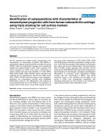
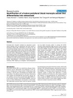
For the case with lower effect size and lower correlation, the
dendrogram resulting from hierarchical cluster analysis is
given in Figure 1. As in the factor analysis, the three groups of
genes clustered together well, although not perfectly. Once
again, however, statistics for determining the appropriate
number of clusters did not clearly identify the correct number
of clusters. The noise genes also seem to follow discernible
clustering patterns. In tight clustering, when the correct
number of clusters are specified and the number of extra clus-
ters (k0) is set to 6-7, 23 of the 90 correlated genes are iden-
tified as noise and all of the noise genes are correctly
identified. Setting the number of clusters higher results in
clusters of noise genes. In this simple case, factor analysis
clearly outperforms both traditional hierarchical cluster anal-
ysis and tight clustering, as it is easily able to discern the cor-
rect number of underlying clusters.
We then increased the number of genes from a total of 190
(90 in the three networks and 100 noise genes) to 1,900 (900
in the three factors and 1,000 noise genes). Using factor anal-

ysis, we easily identified the correct number of factors and
100% of the genes in each factor loaded on the correct factor
(see Table 1). Lowering the correlation among genes in a fac-
tor to ρ = 0.4 resulted in the reduction of the explanatory
power of the factor analysis. The number of underlying fac-
tors was correctly identified although, as expected, the total
variation explained by the factors was reduced. Of the corre-
lated genes, 66% loaded on the correct factors and only one
noise gene (out of 1,000) was mistakenly placed into a factor.
Given the reasonable fractions identified when the number of
genes in factors differs by an order of 10 (190 versus 1,900),
and the fact that our recovery of the structure was virtually
unchanged, it is apparent that the number of genes in a factor
does not impact on the ability of factor analysis to recover the
factor structure. In contrast, hierarchical cluster analysis per-
forms less well as the number of noise genes increases, with
the noise genes increasing in their dispersion among clusters.
In a set of simulations to match our Drosophila experimental
design, 10 genotypes with three replicates per genotype for a
total of 30 samples (chips) were simulated. Averaging tran-
script abundance within each genotype removed
uninteresting variation and increased resolution (data not
shown). We began with three factors of 30 genes each, and
Table 1
Gene expression simulations
Number of
genotypes
Number of factors Number of genes Correlation (ρ) Effect size Factors clearly
identified
Proportion

correct
Noise Each factor
2 3 100 30 0.8 0.2,0.4,0.6 Y 1.00
0.02,0.04,0.06 Y 1.00
0.4 0.2,0.4,0.6 Y 0.84
0.02,0.04,0.06 Y 0.66
2 3 1000 300 0.8 0.2,0.4,0.6 Y 1.00
0.4 0.2,0.4,0.6 Y 0.66
10 3 100 30 0.8 1,2,3 N 0.81
0.4 1,2,3 N 0.64
0 30 0.8 1,2,3 Y 1.00
0.4 1,2,3 N 0.63
10 20 100 30 0.4 1,2, ,20 N -
0.1,0.2, ,2 N -
The number of genotypes simulated is given in the first column. The number of underlying latent factors is given in the second column, followed by
the number of genes simulated that are not a part of any underlying factor. The number of genes on each factor is given next, and are simulated as a
multivariate normal with pairwise correlation among genes within the factor of ρ. The mean for the first genotype is drawn from a gamma
distribution, and the subsequent means were drawn from a multivariate normal, with standard deviation of one such that the maximum difference
between the means can be interpreted as the genotypic effect size. Thus, for each underlying factor the simulated genotypic effect is the maximum
difference in transcript abundance among genotypes for the first, second, and third factor, respectively. Factors are considered to be clearly identified
if there is a substantial drop in the eigenvalues of the correlation matrix, and a reasonable proportion of the total variation is explained. The
proportion correct is the proportion of genes correctly identified when setting the number of factors in the factor analysis to be the simulated
number of latent factors. For the simulation with 20 latent factors we cannot compute the proportion correctly identified, as there are more
simulated factors than possible factors.
R53.4 Genome Biology 2005, Volume 6, Issue 6, Article R53 Coffman et al. />Genome Biology 2005, 6:R53
Figure 1 (see legend on next page)
90
176
23
56

59
145
4
83
15
96
168
174
66
29
162
163
144
122
104
183
134
88
19
31
179
60
102
33
14
166
186
169
62
72

139
78
74
172
69
137
10
165
76
171
141
1
161
79
129
73
115
184
131
50
49
164
126
148
80
180
11
32
124
159

112
77
37
154
67
106
42
97
146
150
6
181
91
47
138
143
58
57
61
157
2
25
140
125
43
30
189
26
86
173

107
3
110
12
123
55
182
151
17
188
41
99
113
111
36
71
118
54
87
20
101
147
7
82
105
75
98
132
8
185

103
133
119
116
156
38
53
120
28
70
177
92
84
24
100
9
170
68
64
65
160
40
94
48
44
109
51
135
93
39

22
35
27
21
89
117
81
155
187
136
190
45
34
175
152
63
121
153
52
16
108
149
5
158
18
128
127
13
178
95

167
130
142
114
46
Genome Biology 2005, Volume 6, Issue 6, Article R53 Coffman et al. R53.5
comment reviews reports refereed researchdeposited research interactions information
Genome Biology 2005, 6:R53
100 noise genes. The maximum difference in transcript abun-
dance among genotypes was large (1, 2 and 3). In this case, the
three factors were not clearly identified. To determine
whether genes would be correctly placed inside factors, the
number of factors was set to three. When difference in tran-
script abundance among genotypes was lowest, fewer genes
were placed in the correct factor (13/30). On the other hand,
where difference in transcript abundance among genotypes
was highest and 100% of the correlated genes loaded on the
correct factor, 29 of the genes from the other two factors and
29 noise genes were erroneously identified as a part of this
factor. When correlation among genes within a factor was
reduced to ρ = 0.40, the difficulty in identifying genes on the
correct factor increased.
We hypothesized that the presence of many noise genes, coin-
cident with a sample size of ten, was responsible for the diffi-
culty in identifying the correct number of gene factors.
Without the noise genes, when correlation was ρ = 0.8, each
of the underlying factors was clearly identified. All (100%) of
the genes were correctly placed in the corresponding factors,
although several genes were placed in multiple factors. When
correlation among genes in a factor was reduced to ρ = 0.40,

the number of factors was underestimated and many of the
genes were identified in multiple factors. This indicates a
complex interplay between the difference in transcript abun-
dance among genotypes, the sample size, the number of noise
genes and the correlation structure in the identification of
factors.
We also examined the impact of increasing the number of fac-
tors beyond the number of genotypes. We simulated a set of
600 genes belonging to 20 factors, with 30 genes in each fac-
tor and 100 noise genes. In an analysis with nine factors (the
maximum estimable with ten genotypes), factor 1 seemed to
capture the majority of all the genes in the 20 factors. When
effect size was large, the majority of the noise genes (58%)
were identified by their failure to load highly (greater than
0.7) on any factor, and the majority of genes that were
correlated did load highly on at least one factor (96%). Low-
ering the correlation lowers the ability to identify correlated
genes as loading highly. In this case, 30% are identified and
approximately the same fraction of noise genes (60%) are
identified. Consistent with previous factor analysis theory
[23,36], when the number of factors is larger than the sample
size the number and composition of the factors cannot be
estimated.
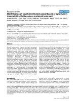
We then wanted to determine whether hierarchical cluster
analysis would resolve this structure more clearly. We plotted
the results in a dendrogram where each of the simulated fac-
tors are plotted with a separate color (Figure 2). No clear pat-
tern of clustering was found. However, the clusters do form
some 'kernels', so that biological knowledge of pathways
could potentially be applied to interpret some of the group-

ings, as is common practice. However, the clear presence of
noise genes throughout the cluster structure clearly makes
interpretation difficult in cases where the true structure is
unknown.
We then applied tight clustering to these data. When the cor-
rect number of clusters is specified, tight clustering does iden-
tify the structure of the 20 clusters. Each cluster consists of a
subset of genes that belong to that cluster. Notably, it does not
erroneously place noise genes into clusters. It performs less
well in identifying the correct number of correlated genes fail-
ing to place 50% into clusters, instead classifying these corre-
lated genes as noise. When a larger number of clusters (25) is
specified, then there are some 'extra' clusters of noise genes
and the clusters of genes are themselves not as distinct, that
is 40 genes of the 600 are incorrectly grouped and 221 or 37%
of the genes which should be in a cluster are designated as
noise.
Overall, the simulation results indicate that focusing on a
manageable number of possible factors with a measurable
amount of difference in transcript abundance among lines
can result in successful identification of factor structure, even
when the number of genes examined is large relative to the
sample size. We also find that the factor loadings can distin-
guish noise genes even in complex cases, although the factor
structure can not be resolved clearly in those cases.
Data analysis
Loci showing evidence for transcript variation
The GeneChip Drosophila Genome Array was used for this
study and of the approximately 13,500 genes on the array,
7,886 showed expression on at least one array, and of these,

4,667 showed evidence for variation among genotypes. As we
are studying covariation, we restricted our examination to
this list of 4,667 loci (see Additional data file 1 [Supplemen-
tary Table 1]).
The immune pathway
To provide an assessment of the performance of factor analy-
sis on a set of well characterized genes, FlyBase [37] was que-
ried for candidate genes involved in the immune pathway
[38]. We compared the candidate genes to the list of 4,667
transcripts, and 54 genes were identified. Factor analysis on
these transcript levels resulted in the identification of three
factors (see Figure 3). Notably, the first factor contained all
the lysogen genes present in the study, and the second factor
Hierarchical cluster plot of simulation with two genotypes, 100 noise genes, and three factorsFigure 1 (see previous page)
Hierarchical cluster plot of simulation with two genotypes, 100 noise genes, and three factors. ρ = 0.40, effect size = 0.2, 0.4, and 0.6. Blue, noise genes;
green, genes from underlying factor 1; red, genes from underlying factor 2; black, genes from underlying factor 3.
R53.6 Genome Biology 2005, Volume 6, Issue 6, Article R53 Coffman et al. />Genome Biology 2005, 6:R53
Figure 2 (see legend on next page)
94
480
294
607
80
380
150
539
183
132
309
439

488
127
140
465
436
391
521
544
338
339
216
459
452
268
162
31
103
552
356
214
241
13
178
647
243
611
15
24
264
440

597
289
192
420
568
626
485
438
506
254
126
266
519
687
78
637
167
328
235
507
429
430
695
500
285
373
177
453
475
402

493
478
16
353
29
615
108
182
518
433
158
434
146
81
341
532
302
352
415
669
118
310
307
653
533
431
350
332
470
358

74
295
407
207
67
649
168
334
395
371
293
203
282
303
419
345
362
113
561
151
683
588
274
154
666
128
2
502
48
87

614
320
437
673
144
105
691
300
681
517
389
357
662
95
688
397
236
290
460
109
259
337
392
564
316
226
139
73
553
161

275
595
117
387
263
71
657
30
383
9
444
620
365
64
79
159
690
446
104
92
410
463
372
694
482
329
20
135
525
643

545
261
678
96
490
616
633
27
37
72
451
34
542
23
277
44
505
276
6
3
651
211
98
83
435
360
398
238
546
426

578
298
297
278
674
333
628
586
331
663
209
200
477
141
652
489
25
405
603
205
305
547
262
36
679
650
422
654
442
110

296
119
54
315
8
670
281
5
416
503
273
265
423
308
38
583
65
499
173
176
60
363
566
249
283
474
388
619
610
385

258
450
199
424
374
70
107
600
101
35
509
515
129
498
335
629
160
364
89
204
621
527
508
432
684
447
665
535
560
233

696
697
642
386
22
257
244
136
291
1
246
312
677
76
123
496
664
571
541
143
689
147
145
215
142
550
198
239
445
396

10
14
582
342
284
443
354
325
301
100
409
222
321
220
675
18
50
692
106
210
590
219
19
99
165
270
401
624
572
327

125
421
116
601
393
340
540
472
556
504
260
85
425
361
33
625
212
685
86
75
102
658
242
299
201
640
412
448
573
534

418
224
237
699
250
55
68
196
4
313
627
458
606
41
636
483
548
172
52
375
511
208
189
469
343
454
218
378
698
481

414
26
591
69
63
115
225
467
77
634
197
667
558
155
529
304
406
656
60
559
230
223
61
351
248
367
623
523
191
62

188
255
114
12
520
476
593
462
494
648
382
497
543
228
660
693
526
580
179
456
492
88
227
441
576
164
630
187
133
149

563
598
252
251
153
175
609
124
562
381
59
58
589
428
399
376
174
53
554
501
355
47
82
323
247
49
90
579
661
130

152
17
166
487
93
646
486
513
46
551
39
682
466
464
400
427
57
569
359
120
148
229
324
193
171
368
186
530
112
522

468
369
314
121
66
346
612
394
231
514
384
565
471
280
267
221
555
491
279
319
567
194
537
170
245
253
700
11
271
51

7
577
330
510
531
288
408
639
287
449
594
234
538
602
269
131
645
479
84
163
21
366
122
286
585
156
336
180
347
599

659
549
581
169
377
390
411
617
181
56
417
240
349
28
457
570
574
272
455
592
461
206
655
512
137
326
575
138
157
322

672
190
584
97
348
43
686
213
635
641
40
306
557
91
631
370
608
344
292
618
473
111
404
195
622
232
45
676
379
42

613
403
495
680
638
668
32
413
632
671
484
317
202
185
217
528
524
318
644
311
256
184
516
536
134
Genome Biology 2005, Volume 6, Issue 6, Article R53 Coffman et al. R53.7
comment reviews reports refereed researchdeposited research interactions information
Genome Biology 2005, 6:R53
contained all cecropins (Table 2). Factor-analysis groups co-
regulated genes in a manner consistent with our understand-

ing of the immune pathway. Hierarchical cluster analysis was
also performed on this set of genes. As with the factor analy-
sis, hierarchical cluster analysis found that the lysogen genes
clustered together, as did the cecropins. However, determin-
ing the appropriate number of clusters was problematic and
did not lead to any clear interpretation of the appropriate
number of clusters. The final factor model for the immune
genes included three factors, therefore we examined a k-
means clustering analysis with three clusters for comparison.
We found that 17/24 (71%) of the genes that loaded high on
factor 1 were on the same cluster. This cluster also includes a
few genes that loaded on factors 2 and 3. Genes that loaded
high on the second and third factor were distributed among
the remaining two clusters. The genes in these groups that did
not load significantly on any factor were distributed among
the three clusters.
Candidate loci for body size
We again queried FlyBase for a list of genes involved in body
size determination and found 92 body size candidates in our
list of 4,667 transcripts. Four factors were identified (Figure
3). The identification of covarying genes in the same factor
was intriguing. Of particular note is the presence of loci that
are contained within quantitative trait loci (QTL) for body
size on factor 1: Cdk4, trx, akt1, fru, Dr, mask, khc, and InR
[33].
In our analysis, we regressed transcript level for individual
candidate genes on the body size phenotype. We found 2,892
genes significant at a nominal level of 0.05 (false discovery
rate (FDR), 16%, see Table 3). At a more stringent nominal
threshold of 0.01, there were 14 candidate genes for body size

which showed significant association between transcript
abundance and phenotypic variation for male body size (FDR
of 7%). Of the QTL candidates, only InR showed significant
association with the phenotype.
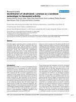
We then tested the hypothesis that the estimated factors were
directly related to phenotypic variation in body size. In our
analysis, we regressed the estimated factor (latent variable)
on the phenotype body size for each genotype. The regression
of factor 1 on body size showed evidence of an association
between the factor and the phenotype of body size (P = 0.04,
Figure 4a).
Hierarchical cluster plot of simulation with ten genotypes, 100 noise genes, and 20 factorsFigure 2 (see previous page)
Hierarchical cluster plot of simulation with ten genotypes, 100 noise genes, and 20 factors. ρ = 0.4, effect size = 1, 2, 20. Blue, noise genes; other colors
represent genes that should cluster together.
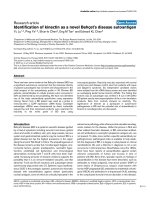
SCREE plotsFigure 3
SCREE plots. The x-axis is the ordinal number of the eigenvalue and the y-axis is the magnitude of the eigenvalue. The number to the right of the plotted
point indicates the cumulative variance explained as each factor is added. The dotted line indicates the cutoff point in the SCREE plot where there is a
sharp drop off in the magnitude of the eigenvalues. The number of factors above the dotted line are the number retained for the factor analysis. (a) Body
size, 92 genes; four factors are selected. (b) Immune, 53 genes; three factors are selected [36].
factor1 (0.25)
factor2 (0.39)
factor3 (0.52)
factor4 (0.63)
factor5 (0.72)
factor6 (0.80)
factor7 (0.88)
factor8 (0.95)
factor9 (1.00)
Four factors selected
factor1 (0.26)

factor2 (0.43)
factor3 (0.58)
factor4 (0.70)
factor5 (0.79)
factor6 (0.86)
factor7 (0.91)
factor8 (0.96)
factor9 (1.00)
Three factors selected
Eigenvalues for body size candidates
Eigenvalues for immune candidates
NumberNumber
5
2
4
6
8
10
12
14
10
0 20 40 60 80 0 10 20 30 40 50
15
20
(a) (b)
R53.8 Genome Biology 2005, Volume 6, Issue 6, Article R53 Coffman et al. />Genome Biology 2005, 6:R53
Targets of miRNAs
Of 535 putative miRNA targets [39], 203 were contained in
our set of 4,667 gene transcripts. Factor analysis resulted in
the identification of four gene factors (Table 4). The second

factor contained four of the same genes as factor 1 for body
size (puc, Eh, mys, bon) with 76 additional genes contained in
this factor (loaded at 0.40 or greater). However, this factor
was not associated with body size (P = 0.55). While some of
the QTL candidates are also putative targets of miRNA
regulation, (Cdk4, trx, Dr) these genes did not participate in
this factor but were common to the factor identified by the
third factor (see Table 4), for which 69 additional genes
loaded. This third factor was negatively correlated with body
size (P = 0.04, see Figure 4b). (Cdk4, trx, Dr) were not asso-
ciated with body size in regressions between these individual
genes and body size.
Discussion
We applied factor analysis to high-dimensional microarray
data. Using simulated data to estimate factors, we found that
when correlation among genes is strong, the number of fac-
tors and their structure can be estimated, even in the case
where genes unrelated to the factor structure (noise genes)
are included. We also found that when noise genes were
included hierarchical cluster analysis was unable to separate
the noise genes from the signal, or to correctly identify the
number of clusters. When the number of genes is large
relative to the sample size, as is common in array studies, the
number of factors and the genes belonging to each factor can
still be identified, as long as the number of factors is less than
the sample size. In contrast, hierarchical cluster analysis did
not identify the number of clusters even when the number of
clusters was smaller than the sample size.
Table 2
Factor analysis for candidate genes for immune function

Factor 1 Factor 2 Factor3
Name Load Name Load Name Load
1 dl 0.93 scrib 0.95 AttB 0.86
2 cact 0.86 CecA1 0.88 GNBP2 0.86
3 LysC 0.86 CecA2 0.85 CG16756 0.85
4 LysD 0.84 IM2 -0.84 CG8193 0.83
5 LysB 0.84 PGRP-SA -0.78 Bc 0.74
6 LysE 0.83 CG5140 -0.76 Eip93F -0.73
7 GNBP3 -0.81 IM1 -0.69 ref(2)P 0.72
8 tub 0.77 IM4 -0.69 CG2736 0.69
9 Tl 0.74 CG6214 0.66 CG3829 0.65
10 CG12780 0.74 CecC 0.63 PGRP-SC2 0.60
11 Mpk2 0.73 PGRP-SC1b -0.59 IM1 -0.59
12 PGRP-LE 0.72 CG1643 -0.53 TepIV 0.53
13 Lectin-galC1 -0.72 PGRP-SD 0.52 CG6214 -0.46
14 LysS 0.70 TepIV -0.51 Drs -0.44
15 CG17338 0.67 cact 0.45 GNBP2 0.43
16 PGRP-SC1a 0.59 Anp 0.44 tub 0.43
17 IM4 -0.56 Lectin-galC1 0.43 Nos 0.42
18 Bc -0.53 Tl 0.41 ref(2)P 0.50
19 ref(2)P 0.50
20 PGRP-SC2 0.49
21 ik2 -0.48
22 BEST:GH02921 -0.48
23 CG3066 0.46
24 CG8193 0.45
Factor analysis for candidate genes for immune function. There were 53 candidate genes and a three-factor model was fitted. The genes that loaded
with a value greater than 0.40 are listed here. For each factor, the first column is the gene symbol name from [37] and the second column is the
loading value for that gene. Genes are considered as loading 'significantly' if the absolute value of the loading value is ≥ 0.40. Genes are considered as
loading 'high' if the absolute value of loading value is ≥ 0.70.

Genome Biology 2005, Volume 6, Issue 6, Article R53 Coffman et al. R53.9
comment reviews reports refereed researchdeposited research interactions information
Genome Biology 2005, 6:R53
We found that if the number of factors is larger than the
number of genotypes, the majority (58%) of noise genes still
do not load on any factor, while all but 26 of the 600 corre-
lated genes do load on at least one factor. However, the cor-
rect association between individual genes and factors is lost.
We conclude that while factor analysis is effective at
separating the signal from the noise, the structure of the sig-
nal is not estimable. This is consistent with reports in the
literature [23,36]. Using hierarchical clustering, the number
and the structure of clusters is not recovered and noise genes
are scattered throughout the cluster structure. Kernels of
tightly correlated genes were visible, however, indicating that
kernel identification is possible in cases where biological
knowledge is present. Any separation of signal from noise is
purely serendipitous.
These results are not unexpected as the mathematical proper-
ties of gene-expression data or the high dimensionality of the
data lead to problems for any analysis. When the number of
columns (in this case observations) is less than the number of
rows (or variables), the matrix is considered ill conditioned
[40]. Ill-conditioned matrices can cause problems for many
types of statistical analysis and can lead to overfitting of pre-
dictive models, among other problems [41,42]. Some of the
effects of the ill-conditioned matrices can be mitigated; how-
ever, the problem of an overdetermined system will always
exist. An example is in multiple regression, where models
with more variables than we have data can not be fit [43].

Tight clustering [27] represents a significant advance over
hierarchical clustering in the estimation of cluster structure
for microarray data. It provides a reasonable way of
identifying most noise genes. In simple cases, however, the
algorithm needs to have some flexibility when specifying
starting values; that is, more rather than fewer clusters
improve the chances of correctly identifying true clusters. The
algorithm requires that the number of clusters be specified a
priori. In contrast, in many simple cases the number and
structure of factors can be recovered precisely using a factor
analysis. In the most complex case examined (20 factors, 600
genes and 100 noise genes), when the number of clusters is
correctly specified, tight clustering identifies 100% of the
noise genes and the 20 clusters with correct genes within each
cluster. However, it also incorrectly identifies 50% of genes
with signal as noise genes. If too many clusters are specified
(25), then the number of genes identified in clusters increases
to 63%, although the correct structure is no longer main-
tained and 20% of the noise genes are incorrectly clustered.
In contrast, factor analysis separates the signal from the
noise, correctly identifying 96% of the noise genes as noise
and 58% of the genes as having signal. In this complex case it
is difficult to say whether factor analysis or tight clustering is
Regression plotsFigure 4
Regression plots. (a) A plot of factor 1 from candidate genes for body size on the x-axis and measured male body size on the y-axis. The solid line is the
regression of factor 1 on measured male body size with an estimated slope of -0.021y with a standard deviation of 0.008 and is significantly different from
zero (P = 0.04). Line crosses: open square 1136; open circle (top left), 611; open triangle 3743; plus sign, 4361; multiplication sign, 6177; open diamond,
g785; inverted open triangle 8599; star 99105; solid circle, 1056; open circle (middle), 3637. (b) A plot of factor 3 from candidate genes for miRNA on the
x-axis and measured male body size on the y-axis. The solid line is the regression of factor 3 on measured male body size with an estimated slope of -
0.020y with a standard deviation of 0.008 and is significantly different from zero (P = 0.04). Symbols as in (a).

Factor 1
Male body size
0.92
0.90
0.88
0.86
0.84
0.82
−3 −2 −1012
Factor 3
−3 −2 −1012
0.92
0.90
0.88
0.86
0.84
0.82
Male body size
(a) (b)
R53.10 Genome Biology 2005, Volume 6, Issue 6, Article R53 Coffman et al. />Genome Biology 2005, 6:R53
Table 3
Factor analysis for candidate genes for body size
Factor 1Factor 2Factor 3Factor 4
Name Load p
1
Name Load p
1
Name Load p
1
Name Load p

1
1 Cdk4 0.98 0.21 l(2)gl -0.90 0.29 Jheh3 -0.97 0.02 dpp 0.79 0.25
2 Kr-h1 0.95 0.01 CkIIbeta 0.86 0.67 cdc2c 0.88 0.21 per 0.72 0.03
3 sqh 0.93 0.02 betaTub
85D
-0.84 0.00 tgo 0.84 0.16 Top1 0.71 0.41
4 trx 0.93 0.26 lilli 0.80 0.09 jar 0.75 0.07 Jheh1 -0.69 0.00
5 babo 0.90 0.00 RpS3 0.78 0.10 Fs(2)Ket 0.75 0.02 wupA 0.65 0.11
6 Akt1 0.88 0.15 Cg25C 0.76 0.13 Sh 0.73 0.11 Fas2 -0.64 0.50
7 fru 0.85 0.13 tra -0.75 0.20 corto 0.72 0.03 Eh -0.62 0.12
8 vg -0.83 0.00 CG1730
9
0.73 0.00 tok -0.67 0.17 tkv 0.62 0.10
9 fng 0.78 0.56 dnc -0.70 0.04 Jheh2 -0.65 0.00 tra 0.62 0.20
10 RpS13 0.72 0.05 mbt 0.69 0.18 woc 0.63 0.32 sbr 0.61 0.15
11 Dp 0.69 0.36 debcl -0.69 0.08 Pi3K92E 0.57 0.12 Jheh2 -0.60 0.00
12 Mef2 0.68 0.06 RpS6 0.66 0.07 qm -0.56 0.26 puc 0.59 0.01
13 Rac2 0.68 0.00 rut 0.64 0.07 aur 0.55 0.02 Nos 0.56 0.02
14 shot 0.65 0.00 ben 0.62 0.24 dare -0.55 0.18 qm 0.56 0.26
15 puc 0.62 0.01 M(2)21A
B
-0.59 0.17 Jheh1 -0.55 0.00 Dr -0.56 0.19
16 M(2)21A
B
0.61 0.17 bon 0.59 0.11 Nos -0.52 0.02 Eip75B 0.53 0.00
17 Dr 0.60 0.19 l(3)mbt 0.58 0.01 hh 0.51 0.04 Pk61C 0.52 0.23
18 trk -0.58 0.27 Pka-C1 0.57 0.55 Pk61C 0.50 0.65 ftz-f1 0.51 0.08
19 Eip75B 0.58 0.00 Eip63E -0.57 0.15 fru 0.50 0.11 CG1191
0
-0.49 0.02

20 fru 0.56 0.11 tkv 0.54 0.10 M(2)21A
B
0.49 0.17 prod -0.47 0.39
21 mask 0.56 0.07 rok -0.54 0.16 mask 0.49 0.07 ninaE -0.47 0.19
22 woc -0.56 0.32 per 0.52 0.03 how 0.49 0.41 dnc 0.45 0.04
23 Dot -0.53 0.11 Sxl 0.50 0.15 neb 0.48 0.74 robl -0.45 0.38
24 Khc 0.53 0.14 neb 0.48 0.74 Egfr -0.47 0.24 InR 0.44 0.01
25 ade2 0.52 0.01 Eh 0.48 0.12 RpS3 -0.47 0.10 vg 0.42 0.00
26 Tsc1 -0.52 0.04 prod -0.47 0.39 mys -0.46 0.11 Pka-C1 -0.41 0.55
27 Fas2 0.51 0.50 wupA 0.47 0.11 robl -0.44 0.38 Khc 0.41 0.14
28 l(3)mbt -0.50 0.01 shot 0.46 0.00 Kr-h1 -0.42 0.01 corto 0.40 0.03
29 Dfd -0.49 0.19 Pk61C -0.44 0.23 Tor 0.41 0.20
30 mys -0.49 0.11 Ddc -0.43 0.19
31 Sh -0.47 0.11 tra2 -0.42 0.24
32 how 0.47 0.41 InR 0.42 0.01
33 Iswi -0.46 0.13 Pi3K92E 0.42 0.12
34 InR 0.45 0.01 hh 0.40 0.04
35 ben 0.44 0.24 Tor 0.40 0.20
36 neb 0.43 0.74
37 Top1 -0.41 0.41
38 tgo -0.40 0.16
Factor analysis for candidate genes for body size. There were 92 candidate genes and a four factor model was fit. The genes that loaded with a value
greater than 0.40 are listed here. For each factor, the first column is the gene symbol name from [37] and the second column is the loading value for
that gene. Genes are considered as loading 'significantly' if the absolute value of the loading value is greater than or equal to 0.40. Genes are
considered as loading 'high' if the absolute value of the loading value is greater than or equal to 0.70. The third column for each factor is the p-value
for the individual gene expression value regression on male body size (p
1
).
Genome Biology 2005, Volume 6, Issue 6, Article R53 Coffman et al. R53.11
comment reviews reports refereed researchdeposited research interactions information

Genome Biology 2005, 6:R53
Table 4
Factor analysis for putative targets of miRNAs
Factor 1 Factor 2 Factor 3 Factor 4
Name Load p
1
Name Load p
1
Name Load p
1
Name Load p
1
1 kel -0.90 0.05 CG5805 -0.92 0.04 CG7995 0.89 0.01 tws 0.80 0.06
2 CG6327 0.89 0.18 Cirl 0.89 0.23 CG4710 0.89 0.07 CG3689 0.78 0.14
3 CG18812 0.88 0.00 CG9245 0.82 0.05 CG4851 0.87 0.19 CG3811 0.77 0.11
4 Cyp314a1 -0.88 0.06 l(2)03709 0.82 0.13 Rpn6 0.87 0.12 CG11883 0.77 0.03
5 Gclc 0.87 0.01 Eh 0.82 0.12 up -0.84 0.24 CG10809 0.74 0.34
6 sima 0.86 0.11 fz 0.81 0.13 Pkc98E 0.82 0.42 CG11128 0.74 0.17
7 CG9924 0.85 0.17 CG6330 0.80 0.11 CSN4 0.80 0.01 CG3961 0.72 0.15
8 CrebA 0.84 0.00 Atpalpha 0.79 0.38 cpo 0.72 0.41 CG5087 0.72 0.06
9 Mbs -0.84 0.04 Surf4 0.79 0.29 drongo 0.72 0.12 unc-13 -0.70 0.07
10 fax 0.79 0.03 sano 0.79 0.02 fng 0.71 0.56 CG12424 0.70 0.16
11 RhoGEF2 0.78 0.11 CG12424 -0.78 0.40 G-oalpha47A 0.70 0.05 CG13344 0.70 0.03
12 CG9664 -0.78 0.34 CG4911 0.78 0.48 PFgn0025879 0.69 0.26 Sap47 0.69 0.05
13 CG2991 0.77 0.12 JhI-21 -0.77 0.34 Cka -0.69 0.12 CG6325 0.69 0.29
14 CG8602 -0.76 0.04 CG9339 0.77 0.09 Ptp99A 0.68 0.07 CG8475 0.68 0.09
15 BicD 0.76 0.07 CG18604 0.76 0.02 cenG1A 0.67 0.22 CG5625 0.67 0.04
16 CG8954 0.76 0.29 G-oalpha47A -0.76 0.02 Ef1gamma 0.67 0.18 PFgn0025879 0.67 0.26
17 dock 0.75 0.08 CG11266 0.76 0.06 CG4452 0.67 0.03 CG5039 0.67 0.01
18 CG10077 0.75 0.03 CG15628 0.75 0.11 CG3764 0.66 0.05 CG3534 -0.67 0.14

19 CG9381 -0.73 0.33 AP-47 0.73 0.15 CG5853 0.66 0.00 Pkc53E 0.65 0.15
20 Mbs 0.72 0.11 CG14762 0.73 0.05 ed 0.65 0.07 CG17646 0.65 0.13
21 BG:DS04929.1 0.71 0.03 CG4963 0.73 0.11 trx 0.65 0.26 CG11178 0.64 0.07
22 bon 0.70 0.11 Eip71CD 0.68 0.09 Cyp18a1 0.64 0.17 CG1814 -0.63 0.00
23 CG9413 0.70 0.60 CG7956 0.67 0.11 SoxN 0.63 0.03 CG14989 0.62 0.07
24 CG6282 -0.69 0.16 ple 0.66 0.17 eIF-5A 0.63 0.23 Sh 0.61 0.11
25 puc 0.69 0.01 CG9297 0.66 0.03 Atpalpha 0.63 0.02 CG9828 0.59 0.20
26 Mkp3 0.68 0.09 CG11198 0.66 0.01 Dr 0.62 0.19 pdm2 -0.58 0.20
27 CG4841 0.68 0.19 Cyp49a1 0.65 0.00 CG3961 0.62 0.15 CG6803 0.58 0.01
28 CG5886 0.67 0.05 gish 0.65 0.04 lack 0.61 0.08 Ptp99A -0.56 0.07
29 CG9934 0.67 0.42 wdp -0.65 0.01 G-oalpha47A -0.61 0.02 Abd-B 0.55 0.06
30 Rab6 0.66 0.09 Pdi 0.65 0.14 CG16971 0.60 0.17 ana 0.55 0.03
31 CG7492 -0.65 0.29 sdk 0.63 0.34 Cdk4 0.60 0.21 CG6199 -0.54 0.26
32 CanA-14F 0.65 0.01 CG4484 -0.63 0.23 CG18854 0.60 0.06 Nmda1 0.54 0.34
33 CG10338 -0.65 0.03 nmdyn-D7 0.62 0.08 aop 0.60 0.01 CG9265 -0.53 0.13
34 CG8617 -0.65 0.22 scrt -0.61 0.17 tws 0.59 0.00 CG10494 0.51 0.26
35 CG6064 0.64 0.01 mys -0.61 0.11 wdp 0.58 0.01 CG9638 0.50 0.05
36 fkh 0.64 0.13 CG11537 0.61 0.33 CG1441 0.57 0.33 RhoGAPp190 0.50 0.00
37 Cka 0.64 0.12 CG8104 0.60 0.07 Cyp49a1 -0.57 0.18 CG4452 0.48 0.03
38 Mkp3 0.62 0.01 Mbs 0.60 0.11 CG17646 0.57 0.02 CG6554 -0.47 0.38
39 trx 0.62 0.26 CG5853 -0.60 0.00 CG4841 0.57 0.19 CG18375 -0.46 0.00
40 CG13586 0.62 0.25 tsl 0.59 0.00 CrebA 0.55 0.10 woc 0.45 0.32
41 amon -0.61 0.21 UbcD2 0.58 0.21 Ef1alpha100E 0.54 0.08 CG8791 0.45 0.03
42 osp 0.60 0.01 ytr 0.58 0.02 Hr39 0.52 0.21 BicD -0.45 0.07
43 Trn 0.60 0.02 G-oalpha47A 0.58 0.05 woc -0.50 0.32 dco 0.44 0.02
44 CG7283 0.60 0.00 CG3800 0.56 0.52 vri 0.50 0.00 amon 0.44 0.21
45 Eip93F 0.59 0.06 Tsf2 0.56 0.21 CG16953 -0.50 0.10 CG1441 -0.44 0.33
46 CrebA 0.59 0.10 BcDNA:LD23587 0.56 0.20 dco -0.49 0.02 CG9297 -0.43 0.03
47 Ptp4E 0.59 0.79 Nmda1 -0.54 0.34 puc 0.49 0.01 CG13586 -0.43 0.25
48 BcDNA:LD32788 0.58 0.13 Ubc-E2H -0.53 0.00 CG8475 0.48 0.09 CG9664 -0.42 0.34

49 Hr39 0.56 0.21 Ac3 0.52 0.23 CG8602 0.48 0.04 scrt 0.41 0.17
50 ed 0.56 0.07 CG15658 -0.51 0.10 CG12424 -0.47 0.16 Cf2 0.41 0.47
51 CG11099 0.56 0.05 bon 0.50 0.11 Asph 0.47 0.02 insc 0.41 0.14
52 sdk -0.56 0.34 sbb 0.49 0.10 BcDNA:LD32788 0.46 0.13 CG4484 0.40 0.23
R53.12 Genome Biology 2005, Volume 6, Issue 6, Article R53 Coffman et al. />Genome Biology 2005, 6:R53
'better'. Both of these approaches clearly outperform hierar-
chical clustering, and they are complementary in their
approach. If the primary goal is to separate the correlated
genes from the uncorrelated genes then factor analysis per-
forms better than tight clustering. If determining the number
and structure of factors (coexpressed genes) is the goal, using
both approaches and comparing findings will be reasonable.
Clear network structures can be identified with factor analysis
and can then be followed up experimentally. Furthermore,
unlike cluster analysis (hierarchical or tight), which provides
no summary of the clusters into a single variable, the factor
loading values are directly interpretable as the degree of par-
ticipation of that locus in a factor. In contrast to cluster anal-
ysis, the factor loadings for genes give us information on the
relative strength of a gene on a factor. We can use factor load-
ings to identify the most 'significant' genes on a factor and we
can use the factor loadings to remove genes that are not con-
tributing to any factor. As such, genes that all load highly on
the same factor can be said to be coordinately expressed and
putatively co-regulated, and noise genes can be identified as
they will not load high on any factor. Unlike clustering, factor
analysis allows genes to participate in several factors, thus
reflecting biological reality more accurately.
Extensions of factor analysis have been developed and
include allowing for nonlinearity [44,45] and the application

of Bayesian approaches [46]. Factor analysis is itself a sub-
class of modeling techniques known as structural equation
models [47] and the ongoing theoretical interest in these
approaches allows for expansion of consideration to more
than the present circumstance.
We focus our Drosophila analyses on a set of genotypes that
are mated according to a round-robin design where the
parental lines are natural variants. Analyses of such lines
allows inferences about the underlying genetic contribution
to variation and inferences about variation in pathways that
53 cenG1A 0.55 0.22 SoxN -0.49 0.03 Cf2 -0.46 0.47 Tsf2 0.40 0.21
54 Vha16 0.54 0.01 aop -0.48 0.01 CG9638 0.46 0.05
55 BcDNA:LD23587 0.54 0.20 CG3764 0.47 0.05 CG14762 -0.46 0.05
56 CG18604 0.54 0.02 CanA-14F 0.47 0.01 CG11266 0.45 0.06
57 Trn 0.52 0.07 CG16953 0.47 0.10 Eip93F -0.44 0.06
58 CG15236 -0.52 0.06 CG15236 -0.47 0.06 CG9413 0.44 0.60
59 fng 0.52 0.56 Trn 0.45 0.02 Abd-B 0.44 0.06
60 did -0.51 0.18 Cka -0.45 0.12 CG6707 0.43 0.75
61 CG11537 0.51 0.33 Ptp4E 0.44 0.79 BcDNA:LD21720 -0.43 0.12
62 CG10494 -0.51 0.26 BG:DS04929.1 0.44 0.03 Cyp49a1 -0.43 0.00
63 CG3534 -0.50 0.14 CG18854 0.44 0.06 CG8791 -0.42 0.03
64 pdm2 -0.50 0.20 vri -0.44 0.00 Sh -0.42 0.11
65 CG8451 -0.50 0.06 CG9924 -0.43 0.17 CG15658 0.42 0.10
66 Eip71CD -0.49 0.09 dco 0.43 0.02 l(2)03709 0.41 0.13
67 gish 0.49 0.04 lack 0.43 0.08 CG6803 0.41 0.01
68 Aef1 -0.49 0.11 CG8791 -0.43 0.03 CG15628 0.41 0.11
69 GLaz 0.48 0.11 CG9664 0.43 0.34 Cyp310a1 -0.41 0.00
70 dco 0.47 0.02 CG5087 -0.43 0.06 BicD -0.41 0.07
71 sbb 0.45 0.10 CG14989 -0.42 0.07 tsl -0.41 0.00
72 BcDNA:LD21720 0.45 0.12 CG6064 0.42 0.01 CG7283 0.40 0.00

73 CG1814 0.44 0.00 CG18375 0.42 0.00
74 CG6199 0.43 0.26 ATPCL 0.41 0.00
75 CG4851 -0.42 0.19 puc -0.41 0.01
76 CG16971 0.41 0.17 CG9638 -0.41 0.05
77 Sap47 0.40 0.05 CG6707 0.41 0.75
78 M(2)21AB 0.40 0.17 CG17646 -0.41 0.02
79 CG4452 0.40 0.03 Atet 0.40 0.08
80 Cf2 -0.40 0.47
Factor analysis for putative targets of miRNAs. There were 203 candidate genes and a four-factor model was fit. The genes that loaded with a value
greater than 0.40 are listed here. For each factor, the first column is the gene symbol name from [37] and the second column is the loading value for
that gene. Genes are considered as loading 'significantly' if the absolute value of the loading value is ≥ 0.40. Genes are considered as loading 'high' if the
absolute value of loading value is ≥ 0.70. The third column for each factor is the the P-value for the individual gene expression value regression on
male body size (p
1
).
Table 4 (Continued)
Factor analysis for putative targets of miRNAs
Genome Biology 2005, Volume 6, Issue 6, Article R53 Coffman et al. R53.13
comment reviews reports refereed researchdeposited research interactions information
Genome Biology 2005, 6:R53
occurs as a result of such natural genetic variation. By using
candidate loci from reverse genetic and mutational projects,
the importance of these loci in a broad context can be
assessed. The factor analysis for the list of genes annotated as
body size candidates resulted in the estimation of four factors.
Factor 1 is of great interest as several of the genes that load on
this factor - Cdk4, trx, akt1, fru, Dr, mask, woc, Khc, and InR
- are contained in QTL for body size [33]. This overlap is excit-
ing as the data from this QTL analyses are independent of our
factor analysis. The identification of the same set of loci lends

weight to the evidence that these loci are involved with the
formation of body size in a natural population. Of these loci,
only InR is directly correlated with body size. Given our lim-
ited knowledge of pathways for body size, it was exciting to
note that two of the genes in this factor - trx and M(2)21AB -
have been shown to interact [48]. In addition, the early sex-
determination cascade genes Sxl, tra, and tra2 are all associ-
ated with a different factor (factor 2).
If the expression of multiple genes is regulated by a common
underlying factor such as a transcription factor or a miRNA,
and this regulation exhibits genetic variation, then we expect
that the gene expression among these genes in a set of geno-
types from a mating design will also be correlated. Factor
analysis on putative targets of miRNA control revealed that
putative targets of the same miRNA often occurred on the
same factor. The number of targets for each miRNA was
small, and so we cannot conclude that the coexpression is
greater than we would expect by chance. Nevertheless, this is
the first opportunity to examine the correlation structure of
these putative targets of miRNAs. We found that of the 203
genes identified as miRNA targets, there was evidence for 188
participating in at least one of the four factors. While four
genes on factor 1 for body size (puc, Eh, mys, and bon), and
nine additional candidate body size genes (Sh, Abd-B, trx,
fng, qm, woc, Dr, and Cdk4) are putative targets of miRNAs
[39], the resulting miRNA factors are uncorrelated with the
factors for body size. One of the miRNA factors is associated
with the body size phenotype.
In summary, factor analysis, a technique developed to dis-
cover and model underlying mechanisms in complex social

and psychiatric situations, seems to offer a reasonable middle
ground for gaining understanding of coordinated gene
expression. Our simulations show that when the number of
underlying factors is larger than the sample size, it is not
straightforward to recover the structure of the simulated data,
although signal can be separated from noise. In contrast,
target groups, even when the number of genes is large, can be
used to identify several underlying regulatory mechanisms.
In the case of body size for Drosophila, factor analysis offers
an exciting opportunity to estimate gene networks, as rela-
tively little is known about how genes involved in body size
work together.
Materials and methods
Simulations
In trying to estimate the structure of gene networks, one of
the first questions to be addressed is whether the number of
genes contributing to each network affects the ability of the
analysis to determine the structure of the network. Accord-
ingly, we varied the number of genes examined in our simula-
tions to explore this process (see Table 1). Gene networks
were simulated as a set of correlated expression values. These
networks represent genes affected by some common underly-
ing biological process and the correlation structure that
results from this biological connectedness is the concrete evi-
dence of the network. In our simulations, for each network, a
mean from a gamma distribution (γ) is drawn. A gamma dis-
tribution was chosen for the mean values across genes as this
distribution has been shown to fit the distribution of tran-
script levels seen from genes on an array [49]. Genes in the
network were simulated according to a multivariate normal

distribution with correlation among genes indicated by the
parameter (ρ). We looked at two levels of correlation ρ = 0.40
(weak) and ρ = 0.80 (strong). Genetic variation for individual
genes within a network was simulated as a linear combination
of the multivariate normal mean, a fixed genotypic effect and
random noise. Genotypic effects for different lines differed in
magnitude. The standard deviation was set to 1, and the
standard normal was used, so that differences between lines
can be directly interpreted as the size of the effect, that is the
effect sizes are absolute and not relative to the magnitude of
the gene expression (or amount of variation) for a particular
gene. When the maximum difference among genotypes is less
than 0.2 the effects are small, when differences are between
0.2 and 0.6 the effects are medium and when effects are larger
than 0.8 they are relatively large [35]. Between networks the
maximum difference of transcript abundance (effect size)
among lines was allowed to vary.
Genes not participating in any network, were also simulated.
These genes, uncorrelated to each other, are hereafter
referred to as noise genes. For noise genes, the mean value for
gene expression was drawn from a gamma distribution and
variation from that mean was random and without regard to
the genotype.
Concurrently, factor analysis on the data was performed and
oblique rotations were used for estimating factor loadings
[36]. We used the eigenvalues to determine the number of
factors according to standard factor analytic approaches [36].
The plot of the eigenvalues, against the ordinal number for
the eigenvalue (SCREE plot) is examined for the last substan-
tial drop in the magnitude of the eigenvalues and a model

with the same number of factors as the number of eigenvalues
before the last substantial drop are retained [23,36]. Hierar-
chical cluster analysis was performed using a Ward distance.
Tight clustering, a resampling-based approach to cluster
analysis, was performed using software provided by [27].
R53.14 Genome Biology 2005, Volume 6, Issue 6, Article R53 Coffman et al. />Genome Biology 2005, 6:R53
Drosophila lines
Isogenic lines of Drosophila simulans were made from flies
caught in Wolfskill orchard [50] and crossed in a round-robin
mating design as follows: the ten parental stocks (randomly
sampled and independently derived from a large natural ref-
erence population) were crossed together in ten combina-
tions to create heterozygous lines such that each parent was
present twice, once as a dam and once as a sire. Crosses were
(dam × sire): SIM6 × SIM11, SIM11 × SIM36, SIM36 × SIM
37, SIM37 × SIM43, SIM43 × SIM61, SIM61 × SIM77, SIM77
× SIM85, SIM85 × SIM99, SIM99 × SIM105, and SIM105 ×
SIM6. The resulting heterozygous genotypes were used for
the experiment as follows: RNA from males was extracted and
labeled 4-7 days post-eclosion [6,50]. Transcript level was
estimated the average difference using MAS 5 [51]. Genes
without positive signal on at least one array were removed
from further consideration. The remaining genes were nor-
malized to the chip median and log transformed. Genes lack-
ing variation among genotypes cannot be meaningfully
assessed for covariation. Accordingly, any gene that showed
evidence (P ≤ 0.2) for variation in transcript level across lines
[50] or evidence for additive genetic effect (P ≤ 0.05) [6] was
considered in further analyses. Adult male flies were meas-
ured for body size [52].

Drosophila data analysis
Candidate gene lists were developed using FlyBase queries.
The miRNA targets were taken from Enright and colleagues
[39]. The resulting lists were matched against the set of loci
for which we had evidence of genetic variation in transcript
abundance among lines.
In the first step of the data analysis, regression of transcript
abundance for individual genes that were candidates for body
size, or putative miRNA targets, was conducted to test the
hypothesis that individual genes transcript levels were associ-
ated with body size. The average transcript abundance for
each gene i within genotype j (g
ij
) was regressed on the aver-
age male body size (Y
j
) for each genotype j as follows:
Y
j
= µ + g
ij
+ ε
ij
. (1)
The mean of all genotypes is µ and the random error is ε. Clus-
ter analysis was performed on the set of immune genes. This
was done using a hierarchical cluster analysis on the stand-
ardized values of gene expression. The results were plotted in
a dendrogram.
Factor analysis on standardized values of gene expression, for

each of the three lists (genes in the immune pathway, candi-
dates for body size and putative miRNA targets) was con-
ducted separately and factor loadings were estimated using
an oblique rotation. The resulting set of eigenvalues was plot-
ted in a SCREE plot, and the number of factors chosen such
that the drop between eigenvalues was apparent, and a rea-
sonable proportion of the variation was explained [36]. Each
factor identified represents a gene network. Once the number
of factors was identified, factor analysis was repeated for that
fixed number of factors and loading values (the correlation
between individual genes and the estimated factor structure)
were estimated. All factor analyses were conducted in SAS
(PROC FACTOR) using standard options, no special coding
was required.
The effect of the factor upon the genotype is also estimable in
the form of a factor value. Factor values were computed as a
linear combination of the factor loading times the standard-
ized value for the gene expression [18,23]. The factor value for
genotype j (GN
j
) is an estimate of the impact of the network
upon the genotype and is estimated as
where g
ij
is the expression value for gene i within genotype j
and l
i
is the loading value estimated from the factor analysis
for gene i across all genotypes. Differences in factor values
represent differences between genotypes for the factor.

As all the genotypes are related in a mating design, we expect
that differences in networks due to genetic variation which
result in phenotypic variation should be detectable. Accord-
ingly, the factor values were then regressed on the phenotype
where
Y
j
= µ + GN
j
+ ε
j
(2)
where GN
j
is the factor value for genotype j.
Additional data files
The following additional data is available with the online ver-
sion of this paper. Additional data file 1 lists the median val-
ues of gene expression for each of the ten lines (after
normalization) for the 4,667 genes found to have some evi-
dence of a line effect. Some basic annotation information
from Affymetrix is also provided along with the feature
number.
Additional File 1Line 1 through Line 10 medians for the 4667 genes considered in this analysis, after normalization (line1
median
) and standardization (line1
median_st
). Some basic annotation is also included as well as the Affymetrix feature number , Fall 2004)Line 1 through Line 10 medians for the 4667 genes considered in this analysis, after normalization (line1
median
) and standardization (line1

median_st
). Some basic annotation is also included as well as the Affymetrix feature number , Fall 2004). The median values of gene expression for each of the ten lines (after normalization) are provided for the 4,667 genes found to have some evidence of a line effect. These are labeled as line1_median-line10_median. Standardized values are also provided and labeled as line1_median _st-line1-_median_st. Some basic annotation information from Affymetrix is also provided along with the feature number. The chromosome number was inferred based upon the cytogenetic map position.Click here for file
Acknowledgements
This work is supported by US Department of Agriculture-IFAFS N0014-94-
1-0318 (L.M.M., C.J.C.), NIH GLUE Grant R24-GM65513 (S.V.N., M.L.W.,
L.M.M.), NIH-NIAID 5R01AI059111-02 (L.M.M.), the Purdue Agricultural
Research Station, the University of Florida Microarray Core Facility, and
the UC Davis Microarray Core Facility. We thank Hayden Bosworth (Duke
University) for introducing us to factor analysis and Chien-Cheng (George)
Tseng for helping us to implement tight clustering.
References
1. Delneri D: The use of yeast mutant collections in genome pro-
filing and large-scale functional analysis. Curr Genomics 2004,
5:59-65.
2. Singh A, McIntyre L, Sherman L: Microarray analysis of the
GN l g
j
i
n
iij
=
∑
´
Genome Biology 2005, Volume 6, Issue 6, Article R53 Coffman et al. R53.15
comment reviews reports refereed researchdeposited research interactions information
Genome Biology 2005, 6:R53
genome-wide response to iron deficiency and iron reconsti-
tution in the cyanobacterium Synechocystis sp. PCC68030.
Plant Physiol 2003, 132:1825-1839.
3. Caldo R, Nettleton D, Wise R: Interaction-dependent gene

expression in Mla-specified response to barley powdery
mildew. Plant Cell 2004, 16:2514-2528.
4. Stern D: Perspective: Evolutionary developmental biology
and the problem of variation. Evolution 2000, 54:1079-1091.
5. Gibson G, Riley-Berger R, Harshman LG, Kopp A, Vacha S, Nuzhdin
SV, Wayne ML: Extensive sex-specific non-additivity in gene
expression in Drosophila melanogaster. Genetics 2004,
167:179-1799.
6. Wayne ML, Pan YJ, Nuzhdin S, McIntyre L: Additivity and trans-
acting effects on gene expression in male Drosophila
simulans. Genetics 2004, 168:1413-1420.
7. Falconer , Mackay T: Introduction to Quantitative Genetics Harlow, UK:
Longman; 1996.
8. Lynch M, Walsh B: Genetics and Analysis of Quantitative Traits Sunder-
land, MA: Sinauer; 1998.
9. Jansen R: Studying complex biological systems using multifac-
torial perturbation. Nat Rev Genet 2003, 4:145-151.
10. Mackay T: The genetic architecture of quantitative traits: les-
sons from Drosophila. Curr Opin Genet Dev 2004, 14:253-257.
11. Adams M, Sekelesky J: From sequence to phenotype: reverse
genetics in Drosophila melanogaster. Nat Rev Genet 2002,
3:189-198.
12. Kalidas S, Smith D: Novel genomic cDNA hybrids produce
effective RNA interference in adult Drosophila. Neuron 2002,
33(2):177-184.
13. Goto A, Blandin S, Royet J, Reichhart J, Levashina E: Silencing of
Toll pathway components by direct injection of double-
stranded RNA into Drosophila adult flies. Nucleic Acids Res 2003,
31:6619-6623.
14. Johnston DS: The art and design of genetic screens: Drosophila

melanogaster. Nat Rev Genet 2002, 3:176-188.
15. Hammond S, Caudy A, Hannon G: Post-transcriptional gene
silencing by double-stranded RNA. Nat Rev Genet 2001,
2:110-119.
16. Fellenberg K, Hauser NC, Brors B, Neutzner A, Hoheisel JD, Vingron
M: Correspondence analysis applied to microarray data. Proc
Natl Acad Sci USA 2001, 98:10781-10786.
17. Wouters L, Gohlmann H, Bijnens L, Kass S, Mohlenbergs G, Lewi P:
Graphical exploration of gene expression data: a compara-
tive study of three gene expression methods. Biometrics 2003,
59:1131-1139.
18. Hatcher L: A Step-by-Step Approach to Using the SAS System for Factor
Analysis and Structural Equation Modeling Cary, NC: SAS; 1994.
19. Wright S: The method of path coefficients. Math Stat 1934,
5:161-215.
20. Dudoit S, Fridlyand J, Speed T: Comparison of discrimination
methods for the classification of tumors using gene expres-
sion data. J Am Stat Assoc 2002, 97:77-87.
21. Tibshirani R, Hastie T, Narasimhan B, Eisen M, Sherlock G, Brown P,
Botstein D: Exploratory screening of genes and cluster from
microarray experiments. Stat Sin 2002, 12:47-59.
22. Parmigiani G, Garrett E, Irizarry R, Zeger S: The analysis of gene
expression data: an overview of methods and software. In The
Analysis of Gene Expression Data Edited by: Parmigiani G, Garrett E,
Irizarry R, Zeger S. New York, NY: Springer; 2003:1-36.
23. Fabrigar L, MacCallum R, Wegener D, Stahan E: Evaluating the use
of exploratory factor analysis in psychological research. Psy-
chol Methods 1999, 4:272-299.
24. Preacher K, MacCallum R: Exploratory factor analysis in behav-
ior genetics research: factor recovery with small sample

sizes. Behav Genet 2002, 32:153-161.
25. Peterson LE: Factor analysis of cluster-specific gene
expression levels from cDNA microarrays. Comput Methods
Programs Biomed 2002, 69:179-188.
26. Peterson LE: CLUSFAVOR 5.0: hierarchical cluster and princi-
pal-component analysis of microarray-based transcriptional
profiles. Genome Biol 2002, 3:software0002.1-0002.8.
27. Tseng G, Wong W: Tight clustering: a resampling-based
approach for identifying stable and tight patterns in data. Bio-
metrics 2005, 61:10-16.
28. Partridge L, French V: Thermal evolution of ectotherm body
size: why get big in the cold. In Animals and Temperature: Pheno-
typic and Evolutionary Adaptation Edited by: Johnston I, Bennett A. Cam-
bridge, UK; Cambridge University Press; 1996:265-296.
29. Huey RB, Gilchrist GW, Carlson ML, Berrigan D, Serra L: Rapid evo-
lution of a geographic cline in size in an introduced fly. Science
2000, 287:308-309.
30. Partridge L, Farquhar M: Lifetime mating success of male fruit-
flies Drosophila melanogaster is related to their size. Animal
Behav 1983, 31:871-877.
31. Partridge L, Mackay T, Aitken S: Male mating success and fertility
in Drosophila melanogaster. Genet Res 1985, 46:279-285.
32. Partridge L, Hoffmann A, Jones JS: Male size and mating success
in Drosophila melanogaster and D. pseudoobscura under field
conditions. Animal Behav 1987, 35:468-476.
33. Caboli F, Kennington W, Partridge L: QTL mapping reveals a
striking coincidence in the positions of genomic regions asso-
ciated with adaptive variation in body size in parallel clines
of Drosophila melanogaster on different continents. Evolution Int
J Org Evolution 2003, 57:2653-2658.

34. Gorsuch R: Factor Analysis 2nd edition. Hillsdale, NJ: Lawrence Erl-
baum Associates; 1983.
35. Cohen J: Statistical Power Analysis for the Behavioral Sciences 2nd edition.
Hillsdale, NJ: Lawrence Erlbaum Associates; 1988.
36. Stevens J: Applied Multivariate Statistics for the Social Sciences Lawrence
Erlbaum Associates; 1996.
37. FlyBase []
38. Andersson M: Sexual Selection Princeton, NJ: Princeton University
Press; 1994.
39. Enright A, John B, Gaul U, Tuschl T, Sander C, Marks D: MicroRNA
targets in Drosophila. Genome Biol 2003, 5:R1.
40. Williams G: Linear Algebra with Applications Boston, MA: Jones and
Bartlett; 2005.
41. Olshen A, Jain A: Deriving quantitative conclusions from
microarray expression data. Bioinformatics 2002, 18:961-970.
42. Hastie T, Tibshirani R, Friedman J: The Elements of Statistical Learning:
Data Mining, Inference, and Prediction New York: Springer; 2001.
43. Neter J, Wasserman W, Kutner M: Applied Linear Statistical Models
New York, NY: McGraw-Hill/Irwin; 1996.
44. McDonald R: Factor interaction in nonlinear factor analysis. Br
J Math Stat Psychol 1967, 20:205-15.
45. Molenaar PC, Boomsma D: Application of nonlinear factor anal-
ysis to genotype-environment interaction. Behav Genet 1987,
17:71-80.
46. Fokoue E, Titterington D: Mixtures of factor analyses. Bayesian
estimation and inference by stochastic simulation. Machine
Learning 2003, 50:73-94.
47. Lee S, Zhu H: Maximum likelihood estimation of nonlinear
structural equation models. Psychometrika 2002, 67:189-210.
48. Gildea J, Lopez R, Shearn A: A screen for new trithorax group

genes identified little imaginal discs, the Drosophila mela-
nogaster homologue of human reinoblastoma binding pro-
tein 2. Genetics 2000, 156:645-663.
49. Black M, Doerge R: Calculation of the minimum number of
replicate spots required for detection of significant gene
expression fold change in microarray experiments. Bioinfor-
matics 2002, 18:1609-1616.
50. Nuzhdin S, Wayne M, Harmon K, McIntyre L: Common patterns
of evolution of gene expression level and protein sequence in
Drosophila. Mol Biol Evol 2004, 21:1308-1317.
51. Affymetrix: Affymetrix GeneChip Expression Analysis Technical Manual
Santa Clara, CA: Affymetrix; 2000.
52. Wayne M, Hackett J, Mackay T: Quantitative genetics of ovariole
number in Drosophila melanogaster. I. Segregating variation.
Evolution 1997, 51:1156-1163.