business economics phần 3 pot
Bạn đang xem bản rút gọn của tài liệu. Xem và tải ngay bản đầy đủ của tài liệu tại đây (218.39 KB, 17 trang )
Introduction to Economics –ECO401 VU
© Copyright Virtual University of Pakistan
36
Arguments like this are frequently used to justify redistributing income and form part of people’s
moral code. Most people would argue that the rich ought to pay more in taxes than the poor and
that the poor ought to receive more state benefits than the rich. The argument is frequently
expressed in terms of a pound being worth more to a poor person than a rich person. It does
not prove that income should be so redistributed, however, unless you argue (a) that the
government ought to increase total utility in society and (b) that it is possible to compare the
utility gained by poor people with that lost by rich people – something that is virtually impossible
to do.
What details does an insurance company require to know before it will insure a person to
drive a car?
Age; sex; occupation; accident record; number of years that a license has been held; traffic law
violations and convictions; model and value of the car; age of the car; details of other drivers of
the car.
How will the following reduce moral hazard?
a. A no-claims bonus.
b. The driver having to pay the first so many rupees of any claim (called “excess”).
c. Offering lower premiums to those less likely to claim (e.g. if a house has a burglar alarm,
it is less likely to be burgled and therefore the insurance premiums for its contents – TV,
VCR, etc. can be reduced by the insurance company).
In the case of (a) and (b) people will be more careful as they would incur a financial loss if the
event they were insured against occurred (loss of no-claims bonus; paying the first so much of
the claim). In the case of (c) it distinguishes people more accurately according to risk. It
encourages people to move into the category of those less likely to claim (but it does not make
people more careful within a category: e.g. those with burglar alarms may be less inclined to turn
them on if they are well insured!).
If people are generally risk averse, why do so many people around the world take part in
national lotteries?
Because the cost of taking part is so little, that they do not regard it as a sacrifice. They also are
likely to take a ‘hopeful’ view (i.e. not based on the true odds) on their chances of winning. What
is more, the act of taking part itself gives pleasure. Thus the behaviour can still be classed as
‘rational’: i.e. one where the perceived marginal benefit of the gamble exceeds the marginal cost.
Why are insurance companies unwilling to provide insurance against losses arising from
war or ‘civil disorder’?
Because the risks are not independent. If family A has its house bombed, it is more likely that
family B will too.
Name some other events where it would be impossible to obtain insurance.
Against losses on the stock market; against crop losses resulting from drought.
Although indifference curves will normally be bowed in toward the origin, on odd
occasions they might not be. What would indifference curves look like in each of the
following cases?
a. X and Y are left shoes and right shoes.
b. X and Y are two brands of the same product, and the consumer cannot tell them
apart.
c. X is a good but Y is a ‘bad’ – like household refuse.
a. L-shaped. An additional left shoe will give no extra utility without an additional right shoe
to go with it!
b. Straight lines. The consumer is prepared to go on giving up one unit of one brand
provided that it is replaced by one unit of the other brand.
Introduction to Economics –ECO401 VU
© Copyright Virtual University of Pakistan
37
c. Upward sloping. If consumers are to be persuaded to put up with more of the ‘bad’, they
must have more of the good to compensate.
What will happen to the budget line if the consumer’s income doubles and the price of
both X and Y double?
It will not move. Exactly the same quantities can be purchased as before. Money income has
risen, but real income has remained the same.
The income–consumption curve is often drawn as positively sloped at low levels of
income. Why?
Because for those on a low level of income the good is not yet in the category of an inferior
good. Take the case of inexpensive margarine. Those on very low incomes may economise on
their use of it (along with all other products), but as they earn a little more, so they can afford to
spread it a little thicker or use it more frequently (the income–consumption curve is positive).
Only when their income rises more substantially do they substitute better quality margarines or
butter.
Illustrate on an indifference diagram the effects of the following: A ceteris paribus (a) rise
in the price of good Y (b) fall in the price of good X.
a. The budget line will pivot inwards from B1 to B2.
b. The budget line would pivot outward on the point where the budget line crosses the
vertical axis. It is likely that the new tangency point with an indifference curve will
represent an increase in the consumption of both goods. The diagram above can be
used to illustrate this. Assume the budget line pivots outwards from B1 to B2. The
optimum consumption point will move from point a to c.
Illustrate the income and substitution effects in the above question.
See the diagram above. In each case the substitution effect is shown by a movement from point
a to point b and the substitution effect is shown by a movement from point b to point c.
Are there any Giffen goods that you consume? If not, could you conceive of any
circumstances in which one or more items of your expenditure would become Giffen
goods?
a
b
c
I
2
I
1
Substitution
Income
Good Y
Good X
B
1
B
1a
B
2
a
b
c
I
2
I
1
Substitution
Income
Good Y
Good X
B
1
B
1a
B
2
(a) Increase in price of Y
(b) Decrease in price of X
Introduction to Economics –ECO401 VU
© Copyright Virtual University of Pakistan
38
It is unlikely that any of the goods you consume are Giffen goods. One possible
exception may be goods where you have a specific budget for two or more items,
where one item is much cheaper: e.g. fruit bought from a greengrocer (or rehri waala
on the street). If, say, apples are initially much cheaper than bananas, you may be able
to afford some of each. Then you find that apples have gone up in price, but are still
cheaper than bananas. What do you do? By continuing to buy some of each fruit you
may feel that you are not eating enough pieces of fruit to keep you healthy and so you
substitute apples for bananas, thereby purchasing more apples than before (but
probably less pieces of fruit than originally).
Introduction to Economics –ECO401 VU
© Copyright Virtual University of Pakistan
39
UNIT - 5
Lesson 5.1
BACKGROUND TO SUPPLY/COSTS
PRODUCTIVE THEORY
A firm is any organized form of production, in which someone or a collection of individuals are
involved in the production of goods and services. A firm can be sole proprietorship (one
person ownership), partnership (a limited number of owners) or a limited company (a large
number of changing shareholders).
A firm is faced with three basic questions:
a. What should it produce?
b. How should it produce it and
c. How much profit/net benefit will the firm make?
The traditional theory of the firm says that the firm’s basic goal is to maximize profits.
Production Function:
A production function is simply the relationship between inputs & outputs.
Mathematically it can be written as:
Q = f (K, L, N, E, T, P……….)
Where,
Q = Output = Total product produced
K = Capital
L = Labor
N = Natural resources
E = Entrepreneurship
T = Technology
P = Power
Cobb Douglas production function:
In economics, the Cobb-Douglas functional form of production functions is widely used to
represent the relationship of an output to inputs. It was proposed by Knut Wicksell, and tested
against statistical evidence by Paul Douglas and Charles Cobb in 1928.
Cobb Douglas production function can be represented by the following equation,
Q = A K
α
L
1 – α
Where:
Q = output
L = labor input
K = capital input
A, α and 1 – α are constants determined by technology.
Short run and Long run:
Short run is a period of time in which at least one of the factors of production is fixed or
unchangeable; long run is a period of time in which all the factors of production used in the
production are flexible. The actual length of the short run and long-run can vary considerably
from industry to industry.
The Law of Diminishing Marginal Returns:
The law of diminishing marginal returns states that as you increase the quantity of a variable
factor together with a fixed factor, the returns (in terms of output) become less and less. Thus
if we are using labor in the production of wheat given a fixed amount of land, after a certain
Introduction to Economics –ECO401 VU
© Copyright Virtual University of Pakistan
40
point the increase in the output of wheat will become less and less until it starts reducing the
total output of wheat.
The total physical product (TPP) of a factor (F) is the latter’s total contribution to output
measured in units of output produced.
Average physical product (APP) is TPP per unit of the variable factor:
APP can be represented by the following formula,
APP = TPPF/QF
Marginal physical product (MPP) is the addition to TPP brought by employing an extra unit
of the variable factor More generally,
MPPF = ∆TPPF/∆QF
Relationship between APP and MPP:
• If the marginal physical product equals the average physical product, the average
physical product will not change.
• If the marginal physical product is above the average physical product, the average
physical product will rise.
• If the marginal physical product is below the average physical product the average
physical product will fall.
Introduction to Economics –ECO401 VU
© Copyright Virtual University of Pakistan
41
Lesson 5.2
BACKGROUND TO SUPPLY/COSTS (CONTINUED………… )
If population is increasing and output remains constant, then diminishing returns set in and
therefore average per capita production/consumption can be expected to fall ceteris paribus.
A firm is confronted with three more decisions;
a. Scale of production,
b. Location, size of industry
c. Optimum combination of inputs.
The Scale of Production:
The scale of production (returns to scale) can be increasing, decreasing or constant.
Increasing (decreasing) returns to scale arise when a 1% increase in the amount of all the
factors employed causes a >1% (<1%) increase in output. Constant returns arise when a 1%
increase in all the factors causes a 1% increase in output.
Returns to scale and returns to factor are two different concepts, the latter related to the short-
term, the former to the long-term.
Increasing returns to scale or (economies of scale) arise if, as firms become bigger and bigger,
their costs per unit of output fall. This could be because of larger more efficient plants, financial
economies, more efficient specialized labour, bulk discounts on purchases etc.
The location, size of Decision:
The location decision depends upon both the location of raw material suppliers and the
location of the market. The nature of the product, transportation costs, availability of suitable
land for production, stable power supply and good communications network, availability of
qualified and skilled workers, level of wages, the cost of local services and availability of
banking and financial facilities are among some other important factors. The size of an
industry can lead to external economies and diseconomies of scale.
External Economies and Diseconomies of Scale:
External economies are benefits accruing to any one firm due to actions or the presence of
other firms. For example, advertising by a rival industry, setting up of credit information
bureaus by banks.
An example of external diseconomies of scale arising is when, as an industry grows larger, a
shortage of specific raw materials or skilled labor occurs, adversely affecting the costs and
prospects of all firms in the industry.
The Optimum Combination of Factors:
The optimum combination of factors will obtain at the point where the marginal physical
product of the last dollar spent on all inputs is equal, i.e.:
MPP
K
= MPP
L
P
K
P
L
Introduction to Economics –ECO401 VU
© Copyright Virtual University of Pakistan
42
Lesson 5.3
BACKGROUND TO SUPPLY/COSTS (CONTINUED………… )
Isoquant:
An isoquant represents different combinations of factors of production that a firm can employ
to produce the same level of output.
Isoquants can be used to illustrate the concepts of returns to scale and returns to factor.
Isoquant Map:
Like an indifference map, an isoquant map consists of parallel isoquants that do not intersect.
The higher the output level the further to the right an isoquant will be.
Marginal Rate of Technical Substitution (MRTS):
The slope of an isoquant is called marginal rate of technical substitution (MRTS). It is
analogous to the term marginal rate of substitution (MRS) in consumer analysis. MRTS is the
amount of one factor, e.g. capital, that can be replaced by a 1 unit increase in the other factor
e.g. labor, if output is to be held constant.
The principle of diminishing MRTS is related to the law of diminishing returns. As one moves
down along an isoquant drawn in K-L space, increasing amounts of labor are used relative to
capital. Now, given diminishing returns, the MPP of labor will fall relative to the MPP of capital.
Isoquants can be used to illustrate the concepts of returns to scale and returns to
factor.
a. Constant returns to scale: equally spaced isoquants;
b. Increasing returns to scale: isoquants become closer and closer to each other;
c. Decreasing returns to scale: isoquants become further and further apart from each
other.
Diminishing returns to factors can be illustrated by keeping one of the inputs constant (say
capital). Here if there are constant returns to scale, ever increasing increments of labor will be
required to produce equal increments to output.
Budget Line:
The concept of isocost is similar to the budget line developed in indifference curve analysis. It
is a line which captures all the different combinations of inputs that the firm can afford to hire.
a. If price of both inputs increases, the isocost line shifts inwards.
b. If price of one input increases, it pivots out.
c. The slope of isocost is PL/PK.
The isoquant-isocost combination can help answer:
a. What is the least cost way of producing a particular level of output?
b. What the highest level of output the firm can produce given a certain budget.
In either case, the optimal factor combination obtains at the point of tangency between the
relevant iso-cost and iso-quant.
Introduction to Economics –ECO401 VU
© Copyright Virtual University of Pakistan
43
Lesson 5.4
BACKGROUND TO SUPPLY/COSTS (CONTINUED………… )
COSTS
Economists argue that sunk cost should not be included in a rational person’s decision making
process while opportunity cost should be included.
Variable Cost and Fixed Costs:
Costs which vary with the level of activity (or output) are called variable costs.
Costs which do not vary with the level of activity or output are called fixed costs. In long run
there are no fixed costs.
There is an inverse relationship between costs and productivity, i.e. as productivity rises,
costs fall and vice versa.
Total Cost:
Total cost (TC) is the sum of all fixed and variable costs. It plot as a vertical summation of the
horizontal line total fixed cost (TFC) curve and the upward sloping total variable cost (TVC)
curve.
Average Cost:
Average cost (AC) is the vertical summation of the AFC & AVC, where
AFC = TFC/Q and
AVC = TVC/Q.
AC = AFC + AVC, where average fixed cost (AFC) is a downward sloping line as you are
dividing a fixed number by an increasing number of output units. By contrast, average variable
cost (AVC) first falls as output increases and then rises.
Study of AC is necessary for firms to be able to set the price or (average revenue) at which
they will sell. Also they will be interested in knowing how AC is broken down into AFC & AVC.
Relationship between AC and AVC:
Initially, AC falls more rapidly than AVC because AC is a summation of AFC & AVC and since
both are falling the effect of two falling curves is greater than the effect of one falling curve.
After the turning point in AVC, both AC and AVC rise but the gap between them narrows
because of same reasoning as given above.
Marginal Cost:
Marginal cost is the addition to TC caused by a unit increase in output. More generally:
MC = ΔTC/ΔQ.
The secret of the shape of the MC curve lies in the law of diminishing marginal returns. The
relationship between MC and AC is a reflection of the relationship between MPP & APP. That
is: both MC and AC fall in the beginning, then MC starts to rise, cutting AC from below at the
latter’s turning point (minima).
In the long run, the law of diminishing marginal returns does not apply to the extent that it does
in short run.
The equivalent of constant, increasing and decreasing returns to scale in terms of costs are
economies of scale, diseconomies of scale and constant costs (or constant returns to scale).
i. In the case of economies of scale, long run total cost (LRTC) is an upward
sloping curve but with falling slope. Note that the slope can never become zero or
negative, though.
ii. In diseconomies of scale, LRTC is an upward sloping curve with an increasing
slope.
Introduction to Economics –ECO401 VU
© Copyright Virtual University of Pakistan
44
iii. In constant costs, LRTC is a positively sloped straight line.
The Long-Run Average Cost Curve (LRAC):
The long-run average cost (LRAC) curve for a typical firm is U shaped.
i. As a firm expands, it initially experiences economies of scale (due to productive
efficiency, better utilization of resources etc.); in other words it faces a downward
sloping LRAC curve.
ii. After the scale of operation is increased further, however, the firm achieve
constant costs i.e., LRAC become flat.
iii. If the firm further increases its scale of operation, diseconomies of scale set in
(due to problems with managing a very large organization etc.) and the LRAC
assumes a positive slope.
The following assumptions are made while deriving LRAC curves:
Price of factors are constant, technology is fixed, firms choose that combination of factors at
which the MPP of the last dollar spent on each input is equal.
Long-run marginal cost (LRMC):
In case a firm is enjoying economies of scale, each incremental unit will cost less than the
preceding one i.e., LRMC will be falling. The opposite will be true for diseconomies of scale. In
case of constant costs, each incremental unit will cost the same, i.e., the LRMC will be
constant.
Relation between SRAC and LRAC curves:
The LRAC curve for a firm is actually derived from its SRAC curves. The exact shape of the
LRAC is a wave connecting the least cost parts of the SRAC curves. In practice however,
LRAC is shown as a smooth U-shaped curve drawn tangent to the SRAC. This is also called
an envelope curve.
Introduction to Economics –ECO401 VU
© Copyright Virtual University of Pakistan
45
Lesson 5.5
BACKGROUND TO SUPPLY/COSTS (CONTINUED………… )
REVENUES
Revenues are the sale proceeds that accrue to a firm when it sells the goods it produces; in
other words they are the cash inflows that the firm received by way of selling its products.
Total Revenue (TR), Average Revenue (AR) and Marginal Revenue (MR):
Total revenue (TR), average revenue (AR) and marginal revenue (MR) concepts apply in the
same way as they did to TC, AC and MC.
i. TR = P x Q.
ii. AR = TR/Q; AR is almost always equal to price unless the firm is engaged in
price discrimination.
iii. MR = ΔTR/ΔQ.
Price-taker and Price-maker Firm:
A firm that does not have the ability to influence market price is a price-taker.
A firm that influences the market price by how much it produces can be called a price-maker or
price-setter.
For a price taker, AR=MR=P. In this case TR is a straight line from the origin. The demand (or
AR) curve the firm faces is a horizontal line.
A price maker faces a downward sloping demand (or AR) curve i.e., it can’t sell more without
reducing price. But this means lowering the price for all units, not just the extra units it hopes
to sell.
The demand faced by a price maker is elastic, when MR is positive and therefore TR
increases due to a decrease in price. Demand is inelastic when MR is negative, and therefore
TR falls due to a decrease in price.
Introduction to Economics –ECO401 VU
© Copyright Virtual University of Pakistan
46
Lesson 5.6
BACKGROUND TO SUPPLY/COSTS (CONTINUED………… )
PROFIT MAXIMISATION
Economists say that when firms earn zero accounting profits, they actually earn normal
economic profits because TC already includes the normal profits that owners of the firms need
for themselves to stay in the business. Positive profits are, for this reason, called supernormal
profits as they are over and above what the owners normally require as a return for their
entrepreneurship.
Approaches of Profit Maximization:
Profit maximization can be studied using the TR-TC approach and the MR-MC approach.
i. In the TR-TC approach it is assumed that firm is price maker and firm is operating
in short run. Total profit is the vertical distance between TR and TC.
ii. In the MR-MC approach, two steps are followed to identify maximum profit. First:
the profit-maximizing output is identified – this is the point where MR cuts MC.
Second: the size of maximum profit is calculated using AC and AR curves.
If MR & AR remain same over the long run, then the profit maximizing output will be obtained
where MR intersects LRMC.
If AC is always above AR, then firms will never be able to make a profit. In this case, the point
where MR=MC, represents the loss-minimizing point.
When MC and MR intersect at two points, not one, then Firms should produce at that point of
intersection of MR and MC beyond which, MC exceeds MR.
If a firm’s AR is below its AVC, it will shut down since it is not covering any part of its fixed
costs.
Profit maximization using calculus:
If total revenue (TR) and total cost equation are given as follows:
TR = 48q – q
2
TC = 12 + 16q + 3Q
2
Then we can find out the value of output at which profit is maximized as under:
Solution:
Profit is maximized at the point where
MC = MR
MC function can be found by taking derivative of total cost function. i.e.:
MC = d TC / dQ
MC = 16 + 6Q
MR function can be found by taking derivative of total revenue (TR) function i.e.:
MR = d TR / dQ
= 48 – 2Q
As profit is maximized at the point where MR = MC, so by equating values of MC and MR
function, we get,
Introduction to Economics –ECO401 VU
© Copyright Virtual University of Pakistan
47
MR =MC
16 + 6Q = 48 – 2Q
6Q + 2Q = 48 – 16
8Q = 32
Q = 4
The equation for total profit is,
Tñ = TR – TC
= 48Q – Q
2
- (12 + 16Q + 3Q
2
)
= 48Q – Q
2
– 12 – 16Q – 3Q
2
= -4Q
2
+ 32Q – 12
Putting Q = 4, we get,
Tñ = - 4(4)
2
+ 32 (4) – 12
= -64 + 128 - 12
Tñ = 52
So profit is maximized where output is 4 and the maximum profit is 52.
Introduction to Economics –ECO401 VU
© Copyright Virtual University of Pakistan
48
END OF UNIT 5 - EXERCISES
How will the length of the short run for a shipping company depend on the state of the
shipbuilding industry?
If the shipbuilding industry is in recession, the short run (and the long run) may be shorter. It
will take less time to acquire a new ship if there is no waiting list, or if there are already ships
available to purchase (with perhaps only minimal modifications necessary).
Up to roughly how long is the short run in the following cases?
(a) A mobile ice-cream firm. (b) A small grocery. (c) Electricity power generation.
a) 2-3 days: the time necessary to acquire new bicycles, equipment and workers.
b) Several weeks: the time taken to acquire additional premises.
c) 3-5 years: the time taken to plan and build a new power station.
How would you advise the naanwaala (bread-maker) next door as to whether he should
(a) employ an extra assistant on a Sunday (which is a high demand day); (b) extend his
shop, thereby allowing more customers to be served on a Sunday?
a) If maximizing profit is the sole aim, then he should employ an additional assistant if the
extra revenue from the extra customers that the assistant can serve is greater than the
costs of employing the assistant.
b) Only if the extra revenue from the extra customers will more than cover the costs of the
extension plus the extra staffing.
Given that there is a fixed supply of land in the world, what implications can you draw
from about the effects of an increase in world population for food output per head?
Other things being equal, diminishing returns would cause food output per head to decline (a
declining MPP and APP of labour). This, however, would be offset (partly, completely or more
than completely) by improvements in agricultural technology and by increased amounts of
capital devoted to agriculture: this would have the effect of shifting the APP curve upwards.
The following are some costs incurred by a shoe manufacturer. Decide whether each
one is a fixed cost or a variable cost or has some element of both.
(a) The cost of leather. (b) The fee paid to an advertising agency. (c) Wear and tear on
machinery. (d) Business rates on the factory. (e) Electricity for heating and lighting. (f)
Electricity for running the machines. (g) Basic minimum wages agreed with the union.
(h) Overtime pay. (i) Depreciation of machines as a result purely of their age
(irrespective of their condition).
(a) Variable. (b) Fixed (unless the fee negotiated depends on the success of the campaign).
(c) Variable (the more that is produced, the more the wear and tear). (d) Fixed. (e) Fixed if
the factory will be heated and lit to the same extent irrespective of output, but variable if the
amount of heating and lighting depends on the amount of the factory in operation, which in
turn depends on output. (f) Variable. (g) Variable (although the basic wage is fixed per
worker, the cost will still be variable because the total cost will increase with output if the
number of workers is increased). (h) Variable. (i) Fixed (because it does not depend on
output).
Assume that a firm has 5 identical machines, each operating independently. Assume
that with all 5 machines operating normally, 100 units of output are produced each day.
Below what level of output will AVC and MC rise?
20 units. Below this level, the one remaining machine left in operation will begin to operate at a
level below its optimum. (Note that with 5 machines producing 100 units of output, minimum
AVC could be achieved at 100, 80, 60, 40 and 20 units of output, but between these levels
some machines may be working at less than their optimum and some at more than their
Introduction to Economics –ECO401 VU
© Copyright Virtual University of Pakistan
49
optimum. Thus if the optimum level for a machine is critical, then the AVC curve may look
‘wavy’ rather than a smooth line.
Why is the minimum point of the AVC curve (y) at a lower level of output than the
minimum point of the AC curve (z)?
Because between points y and z marginal cost is above AVC (and thus AVC must be past the
minimum point) but below AC (and thus AC cannot yet have reached the minimum point).
Even though AVC is rising beyond point y, the fall in AFC initially more than offsets the rise in
AVC and thus AC still falls.
What economies of scale is a large department store likely to experience?
Specialized staff for each department (saving on training costs and providing a more efficient
service for customers); being able to reallocate space as demand shifts from one product to
another and thereby reducing the overall amount of space required; full use of large delivery
lorries which would be able to carry a range of different products; bulk purchasing discounts;
reduced administrative overheads as a proportion of total costs.
Why are firms likely to experience economies of scale up to a certain size and then
diseconomies of scale after some point beyond that?
Because economies of scale, given that most arise from increasing returns to scale, will be
fully realized after a certain level of output, whereas diseconomies of scale, given that they
largely arise from the managerial problems of running large organizations, are only likely to set
in beyond a certain level of output.
How is the opening up of trade and investment between, say eastern and western
Europe, likely to affect the location of industries within Europe that have (a) substantial
economies of scale; (b) little or no economies of scale?
a) Given that production will take place in only one or two plants, new plants will tend to
be located near to the centre of the new enlarged European market.
b) Plants will still tend to be scattered round Europe, given that the customers are
scattered.
These effects will be the result of attempts to minimize transport costs and thus will be more
significant the higher are transport costs per kilometer.
Name some industries where external economies of scale are gained. What are the
specific external economies in each case?
Two examples are:
• Financial services: pool of qualified and experienced labour, access to specialist
software, one firm providing specialist services to another.
• Various parts of the engineering industry: pool of qualified and experienced labour,
access to specialist suppliers, possible joint research, specialized banking services.
Would you expect external economies to be associated with the concentration of an
industry in a particular region?
Yes. There may be a common transport and communications infrastructure that can be used;
there is likely to be a pool of trained and experienced labour in the area; joint demand may be
high enough to allow economies of scale to be experienced in the supply of some locally
extracted raw material.
If factor X costs twice as much as factor Y (Px/Py = 2), what can be said about the
relationship between the MPPs of the two factors if the optimum combination of factors
is used?
MPPx/MPPy = 2. The reason is that if MPPx/Px = MPPy/Py, then, by rearranging the terms of
the equation, MPPx/MPPy must equal Px/Py (= 2).
Introduction to Economics –ECO401 VU
© Copyright Virtual University of Pakistan
50
Could isoquants ever cross?
Not for a given state of technology, otherwise it would mean that at one side of the intersection
the higher output isoquant would be ‘south-west’ of the lower output isoquant. This would
mean that a higher output could be achieved by using less of both factors of production!
Could they ever slope upward to the right?
Yes. It would mean that one of the two factors had a negative marginal productivity that was
greater than the positive marginal productivity of the other: i.e. that MPPa/MPPb (or
MPPb/MPPa) was negative (a negative marginal rate of factor substitution).
This situation will occur when so much is used of one factor that diminishing returns have
become so great as to produce substantial negative marginal productivity: isoquants will bend
back on themselves beyond the points where they become vertical or horizontal. The firm,
however, will not produce along this portion of an isoquant, because the price ratio (Pa/Pb) will
(virtually) never be negative.
What will happen to an isocost if the prices of both factors rise by the same
percentage?
It will shift inwards parallel to the old isocost.
Why do the prices of cattle and sheep prices fall so drastically “on”, or just “after” the
first day of Eid-ul-Azha?
The supply curve for cattle and sheep is fixed in the short-run, i.e. a vertical supply curve,
therefore price will be determined by demand. Since demand for “cattle for sacrifice” falls
drastically after or on the first day of Eid-ul-Azha, the price has to come down drastically as
well for the market to clear.
Explain the shape of the LRMC curve for a firm with a typical U-shaped LRAC curve.
At first economies of scale cause the LRMC to fall. Then because of (marginal) diseconomies
of scale, additional units of production begin to cost more to produce than previous units: the
LRMC begins to slope upwards. But the LRAC is still falling because the LRMC is below it
pulling it down. It is not until the LRMC crosses the LRAC that the firm will experience a rising
LRAC and hence average diseconomies of scale.
Will the “envelope curve” be tangential to the bottom of each of the short-run average
cost curves? Explain why it should or should not be.
No. At the tangency points the two curves must have the same slope. Thus the slope at the
tangency point is not zero (the slope at the turning point or minima of the SRAC curves).
What would the isoquant map look like if there were (a) continuously increasing returns
to scale; (b) continuously decreasing returns to scale?
a) The isoquants would get progressively closer and closer together.
b) The isoquants would get progressively further and further apart.
What can we say about the slope of the TR and TC curves at the maximum profit point?
What does this tell us about marginal revenue and marginal cost?
The slopes are the same. But given that the slope of the total curve gives the respective
marginal, this means that marginal revenue will be equal to marginal cost.
Introduction to Economics –ECO401 VU
© Copyright Virtual University of Pakistan
51
Fill in the missing figures in the table below.
Q P =
AR
TR MR TC AC MC
T
Π
A
Π
0 9 6
1 8 10
2 7 12
3 6 14
4 5 18
5 4 25
6 3 36
7 2 56
Q P = AR TR MR TC AC MC
T
Π
A
Π
0 9 0 6 – –6 –
8 4
1 8 8 10 10 –2 –2
6 2
2 7 14 12 6 2 1
4 2
3 6 18 14 4.3 4 1.3
2 4
4 5 20 18 4.5 2 0.5
0 6
5 4 20 25 5 –5 –1
–2 9
6 3 18 36 6 –18 –3
–4 16
7 2 14 56 8 –42 –6
Why should the figures for MR and MC be entered in the spaces between the lines?
Because marginal revenue (or cost) is the extra revenue (or cost) from moving from one quantity
to another.
Introduction to Economics –ECO401 VU
© Copyright Virtual University of Pakistan
52
You are given the following information for a firm.
Q 0 1 2 3 4 5 6 7
P 12 11 10 9 8 7 6 5
TC 2 6 9 12 16 21 28 38
Construct a detailed table like the one you constructed in the earlier question with TR, AC,
MR, TC, AC, MC, TΠ and AΠ. Use your table to draw “two” diagrams (one with the marginal
revenue and cost curves, and one with the total (or average) revenue and cost curves) and
use them to show the “profit-maximising output” and the “level of maximum profit”,
respectively. Confirm your findings by reference to the table you construct.
Q P = AR TR MR TC AC MC
T
Π
A
Π
0 12 0 2 – –2 –
11 4
1 11 11 6 6 5 5
9 3
2 10 20 9 4.5 11 5.5
7 3
3 9 27 12 4 15 5
5 4
4 8 32 16 4 16 4
3 5
5 7 35 21 4.2 14 2.8
1 7
6 6 36 28 4.7 8 1.3
–1 10
7 5 35 38 5.4 –3 –0.4
The curves will be a similar shape to those discussed in the lecture, and included in the slides
handout. The peak of the TΠ curve will be at Q = 4. This will be the output where MR and MC
intersect.
Will the size of normal ‘profit’ vary with the general state of the economy?
Yes. Normal profit is the rate of profit that can be earned elsewhere (in industries involving
similar level of risk). When the economy is booming, profits will normally be higher than when
the economy is in recession. Thus the ‘normal’ profit that must be earned in any one industry
must be higher to prevent capital being attracted to other industries.
Given the following equations:
TR = 72Q – 2Q²; TC = 10 + 12Q + 4Q²
Calculate the maximum profit output and the amount of profit at that output using both
methods.
(a) TΠ = 72Q – 2Q² – 10 – 12Q – 4Q
= –10 + 60Q – 6Q² (1)
∴ dTΠ /dQ = 60 – 12Q
Setting this equal to zero gives: