Managerial economics theory and practice phần 2 doc

DERIVATIVE OF A FUNCTION
Consider, again, the function
(2.1)
The slope of this function is defined as the change in the value of y divided
by a change in the value of x, or the “rise” over the “run.” When defining
the slope between two discrete points, the formula for the slope may be
given as
(2.6)
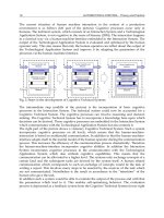
Consider Figure 2.12, and use the foregoing definition to calculate the
value of the slope of the cord AB. As point B is brought arbitrarily closer
to point A, however, the value of the slope of AB approaches the value of
the slope at the single point A, which would be equivalent to the slope of
a tangent to the curve at that point. This procedure is greatly simplified,
however, by first taking the derivative of the function and calculating its
value, in this case, at x
1
.
The first derivative of a function (dy/dx) is simply the slope of the func-
tion when the interval along the horizontal axis (between x
1
and x
2
) is made
infinitesimally small.Technically,the derivative is the limit of the ratio Dy/Dx
as Dx approaches zero, that is,
(2.44)
When the limit of a function as x Æ x
0
equals the value of the function at
x
0

, the function is said to be continuous at x
0
, that is, lim
xÆx
0
f(x) = f(x
0
).
dy
dx
y
x
x
=
Ê
Ë
ˆ
¯
Æ
lim
D
D
D
0
Slope =
=
-
-
=
()

-
()
-
D
D
y
x
yy
xx
fx fx
xx
21
21
21
21
yfx=
()
62 introduction to mathematical economics
y= f(x)
y
x
0 x
1
x
2
y
2
y
1
A

B
FIGURE 2.12 Discrete versus instanta-
neous rates of change.
Calculus offers a set of rules for using derivatives (slopes) for making
optimizing decisions such as minimizing cost (TC) or maximizing total
profit (p).
RULES OF DIFFERENTIATION
Having established that the derivative of a function is the limit of the
ratio of the change in the dependent variable to the change in the inde-
pendent variable, we will now enumerate some general rules of differenti-
ation that will be of considerable value throughout the remainder of this
course. It should be underscored that for a function to be differentiable at
a point, it must be well defined; that is it must be continuous or “smooth.”
It is not possible to find the derivative of a function that is discontinuous
(i.e., has a “corner”) at that point. The interested student is referred to
the selected adings at the end of this chapter for the proofs of these
propositions.
POWER-FUNCTION RULE
A power function is of the form
where a and b are real numbers. The rule for finding the derivative of a
power function is
(2.45)
where f¢(x) is an alternative way to denote the first derivative.
Example
A special case of the power-function rule is the identity rule:
Another special case of the power-function rule is the constant-function
rule. Since x
0
= 1, then
yfx ax a=

()
==
0
dy
dx
fx x x=¢
()
=
()
==
-
11 1 1
11 0
yfx x=
()
=
dy
dx
fx x x=
¢
()
=
()
=
-
24 8
21
yx= 4
2
dy

dx
f x bax
b
=¢
()
=
-1
yfx ax
b
=
()
=
rules of differentiation 63
Thus,
Example
SUMS AND DIFFERENCES RULE
There are a number of economic and business relationships that are
derived by combining one or more separate, but related, functions. A firm’s
profit function, for example, is equal to the firm’s total revenue function
minus the firm’s total cost function. If we define g and h to be functions of
the variable x, then
(2.46)
Example
Example
a. Consider the general case of the linear function
(2.5)
b. y = f(x) = 5 - 4
c. From Problem 2.1
QP
S

=+10 2
QP
D
=-25 3
dy
dx
fx=
¢
()
=-4
dy
dx
fx
du
dx
dv
dx
bb=
¢
()
=+=+=0
yfx gxhx abx=
()
=
()
+
()
=+
dy
dx

fx x=
¢
()
=+22
yfx gxhx xx=
()
=
()
+
()
=+2
2
ugx xvhx x=
()
==
()
=2
2
;
dy
dx
fx
du
dx
dv
dx
=¢
()
=±
yfx uvgxhx=

()
=±=
()
±
()
ugxvhx=
()
=
()
;
dy
dx
fx=
¢
()
=◊
()
=
-
01 5 0
01
y ==◊515
0
dy
dx
fx ax=¢
()
=
()
=

-
00
01
64 introduction to mathematical economics
Example
PRODUCT RULE
Similarly, there are many relationships in business and economics
that are defined as the product of two or more separate, but related, func-
tions. The total revenue function of a monopolist, for example, is the
product of price, which is a function of output, and output, which is a func-
tion of itself. Again, if we define g and h to be functions of the variable x,
then
Further, let
Although intuition would suggest that the derivative of a product is the
product of the derivatives, this is not the case. The derivative of a product
is defined as
(2.47)
Example
Substituting into Equation (2.47)
dy
dx
fx x x x x x=
¢
()
=-
()
+-
()()
=- +22324 1212
22

dv
dx
hx=
¢
()
=-2
vx=-
()
32
du
dx
gx x=
¢
()
= 4
ugx x=
()
= 2
2
yx x=-
()
232
2
dy
dx
fx u
dv
dx
v
du

dx
uh x vg x=¢
()
=
Ê
Ë
ˆ
¯
+
Ê
Ë
ˆ
¯
=¢
()
+¢
(
)
yfx uvgxhx=
()
==
()
◊
()
ugxvhx=
()
=
()
;
dy

dx
fx x x=
¢
()
=-+012 18 1
0
2

yxxx=-++004 09 10 5
32

dQ
dP
S
= 2
dQ
dP
D
=-3
rules of differentiation 65
QUOTIENT RULE
Even less intuitive than the product rule is the quotient rule. Again,
defining g and h as functions of x, we write
Further, let
then
(2.48)
Example
Substituting into Equation (2.48), we have
Interestingly, in some instances it is convenient, and easier, to apply the
product rule to such problems. This becomes apparent when we remember

that
Example
yfx
gx
hx
x
x
xx x x=
()
=
()
()
==
()
=
()
[]
-
-
2
3
23 2 13
2
2
1
21
y
u
v
uv==

-1
dy
dx
fx
xxx
x
xx
x
x
x
=
¢
()
=
-
()

()
()
=
-
=
-22324
2
412
4
3
2
2
2

2
43
dv
dx
hx x=
¢
()
= 4
vhx x=
()
= 2
2
du
dx
gx=
¢
()
=-2
ugx x=
()
=-32
yfx x x=
()
=-
()
32 2
2
dy
dx
fx

v du dx u dv dx
v
h x dg x dx g x dh x dx
hx
hx g x gx h x
hx
=¢
()
=
()
-
()
=
() ()
[]
-
() ()
[]
()
=
()
ע
()
-
()
ע
()
()
2
2

2
yfx
u
v
gx
hx
=
()
==
()
()
ugxvhx=
()
=
()
;
66 introduction to mathematical economics
It is left to the student to demonstrate that the same result is derived by applying
the quotient rule.
CHAIN RULE
Often in business and economics a variable that is a dependent variable
in one function is an independent variable in another function. Output Q,
for example, is the dependent variable in a perfectly competitive firm’s
short-run production function
where L represents the variable labor, and K
0
represents a constant amount
of capital labor utilizes in the short run. On the other hand, output is the
independent variable in the firm’s total revenue function
where P is the (constant) selling price.

In the example just given, we might be interested in determining how
total revenue can be expected to change given a change in the firm’s labor
usage. For this we require a technique for taking the derivative of one func-
tion whose independent variable is the dependent variable of another func-
tion. Here we might be interested in finding the derivative dTR/dL. To find
this derivative value, we avail ourselves of the chain rule. Let y = f(u) and
u = g(x). Substituting, we are able to write the composite function
The chain rule asserts that
(2.49)
Applying the chain rule, we get
Example
yfu u=
()
=+
3
10
yx=
()
+210
2
3
dTR
dL
dTR
dQ
dQ
dL
LL L=
Ê
Ë

ˆ
¯
Ê
Ë
ˆ
¯
=
()
==

10 2 20 20
05 05
dy
dx
dy
du
du
dx
df u
du
dg x
dx
fu gx
=
Ê
Ë
ˆ
¯
Ê
Ë

ˆ
¯
=
()
È
Î
Í
˘
˚
˙
()
È
Î
Í
˘
˚
˙
=¢
()
ע
()
yfgx=
()
[]
TR g Q PQ Q=
()
==10
QfLK L=
()
=,

.
0
05
4
dy
dx
fx x x x x=
¢
()
=-
()
[]
+
()()
=- + =

2 13 13 4 23 43 23
22 1
rules of differentiation 67
EXPONENTIAL AND LOGARITHMIC FUNCTIONS
Now we consider the derivative of two important functions–the expo-
nential function and the logarithmic function. The number e is the base of
the natural exponential function, y = e
x
. The natural logarithmic function is
y = log
e
x = ln x. The number e is itself generated as the limit to the series
(2.50)
To illustrate the practical importance of the number e, suppose, for

example, that you were to invest $1 in a savings account that paid an inter-
est rate of i percent. If interest was compounded continuously (see Chapter
12), the value of the deposit at the year end would be
(2.51)
Now, suppose that a deposit of D dollars was compounded continuously
for n years. At the end of n years the deposit would be worth
The derivative of the exponential function y = e
x
is
(2.52)
That is, the derivative of the exponential function is the exponential func-
tion itself.
The derivative of the natural logarithm of a variable with respect to
that variable, on the other hand, is the reciprocal of that variable. That
is, if
then
y
x
e
= log
dy
dx
de
dx
e
x
x
=
()
=

lim lim
h
h
in
h
n
t
in
D
h
D
h
De
Æ• Æ•
+
Ê
Ë
ˆ
¯
È
Î
Í
˘
˚
˙
=+
Ê
Ë
ˆ
¯

È
Î
Í
˘
˚
˙
=1
1
1
1
lim
h
h
i
i
h
e
Æ•
+
Ê
Ë
ˆ
¯
=1
e
h
h
h
=+
Ê

Ë
ˆ
¯
=
Æ•
lim . . . .1
1
2 71829
dy
dx
fx u x x x x x x=
¢
()
=
()
=
()
◊
()
=◊=3 4 3 2 2 4 12 4 48
22
2
4
5
du
dx
gx x=
¢
()
= 4

ugx x=
()
= 2
2
dy
du
fu u x x=
¢
()
==
()
=332 12
22
2
4
68 introduction to mathematical economics
(2.53)
When more complicated functions are involved, we can apply the chain
rule. Suppose, for example, that y = ln x
2
. Letting u = x
2
this becomes
y = ln u. The derivative of y with respect to x then becomes
It may also be demonstrated that the result for the derivative of an expo-
nential function follows directly from a special relationship that exists
between the exponential function and the logarithmic function. Given the
function x = e
y
, then y = ln x. Moreover, if x = ln y, then y = e

x
. These func-
tions are said to be reciprocal functions. When two functions are related in
this way, the derivatives are also related; that is, dy/dx = 1/(dx/dy). Using
this rule, we can prove the exponential function rule:
Returning to the earlier discussion of continuous compounding, suppose
that the value of an asset is given by
where r is the rate of interest, t time, and D the initial value of the asset.
The rate of change of the value of the asset over time is
That is, the rate of change in the value of the asset is the rate of interest
times the value of the asset at time t.
INVERSE-FUNCTION RULE
Earlier in this chapter we discussed the existence of inverse functions. It
will be recalled that if the function y = f(x) is a one-to-one correspondence,
then not only will a given value of x correspond to a unique value of y, but
a given value of y will correspond to a unique value of x. In this case, the
function f has the inverse function g(y) = f
-1
(y) = x, which is also a one-to-
one correspondence. Given an inverse function, its derivative is
dDe
dt
D
de
dt
e
dD
dt
D
de

du
du
dt
e
dD
dt
De r e rDe
rt rt
rt
u
rt
urt rt
()
=
Ê
Ë
ˆ
¯
+
Ê
Ë
ˆ
¯
=
Ê
Ë
ˆ
¯
Ê
Ë

ˆ
¯
+
Ê
Ë
ˆ
¯
=+
()
=0
Dt De
rt
()
=
de
dx
dy
dx d y dy y
ye
x
x
()
==
()
===
11
1ln
dy
dx
dy

du
du
dx
ux
x
x
x
=
Ê
Ë
ˆ
¯
Ê
Ë
ˆ
¯
=
()()
=
Ê
Ë
ˆ
¯
()
=12
1
2
2
2
dy

dx
dx
dx x
e
=
()
=
log 1
rules of differentiation 69
(2.54)
Equation (2.54) asserts that the derivative of an inverse function is the
reciprocal of the derivative of the original function.
It will also be recalled that functions with a one-to-one correspondence
are said to be monotonically increasing if x
2
> x
1
fi f(x
2
) > f(x
1
). Functions
in which a one-to-one correspondence exist are said to be monotonically
decreasing if x
2
> x
1
fi f(x
2
) < f(x

1
). In general, for an inverse function to
exist, the original function must be monotonic. In other words, it is not
possible to write x = g(y) = f
-1
(y) until we have determined whether the
function y = f(x) is monotonic.
It is possible to determine whether a function is monotonic by examin-
ing its first derivative. If the first derivative of the function is positive for all
values of x, then the function y = f(x) is monotonically increasing. If the first
derivative of the function is negative for all values of x, then the function
y = f(x) is monotonically decreasing.
Problem 2.5. Consider the function
a. Is this function monotonic?
b. If the function is monotonic, use the inverse-function rule to find
dx/dy.
Solution
a. The derivative of this function is
which is positive for all values of x. Thus, the function f(x) is a monoto-
nically increasing function.
b. Because f(x) is a monotonically increasing function, the inverse function
g(y) = f
-1
(y) exists. Thus, it is possible to use the inverse-function rule to
determine the derivative of the inverse function, that is,
It should be noted that the inverse-function rule may also be applied to
nonmonotonic functions, provided the domain of the function is restricted.
For example, y = f(x) = x
2
is nonmonotonic because its derivative does not

have the same sign for all values of x. On the other hand, if the domain of
this function is restricted to positive values for x, then dy/dx > 0.
dx
dy dy dx
xx
==
++
11
47
46
dy
dx
fx x x=¢
()
=+ +47
46
yfx x x x=
()
=+ +402
57
.
¢
()
== =
¢
()
gy
dx
dy dy dx f x
11

70 introduction to mathematical economics
Problem 2.6. Consider the function
a. Is this function monotonic?
b. If the function is monotonic, use the inverse-function rule to find dx/dy.
Solution
a. The derivative of this function is
This function is not monotonic, since the sign of dy/dx depends on
whether x is positive or negative. On the other hand, the derivative is
negative for all positive values for x.
b. Because the derivative of f(x) is positive for all x > 0, then it is possible
to use the inverse-function rule to determine the derivative of the inverse
function, that is,
for all x > 0.
IMPLICIT DIFFERENTIATION
The functions we have been discussing are referred to as explicit func-
tions. Explicit functions are those in which the dependent variable is on the
left-hand side of the equation and the independent variables are on the
right-hand side. In many cases in business and economics, however, we may
also be interested in what are called implicit functions.
Implicit functions are those in which the dependent variable is also func-
tionally related to one or more of the right-hand-side variables. Such func-
tions often arise in economics as a result of some equilibrium condition that
is imposed on a model. A common example of an implicit function in
macroeconomic theory is in the definition of the equilibrium level of
national income Y, which is given as the sum of consumption spending C,
which is itself assumed to be a function of national income, net investment
spending I, government expenditures G, and net exports X - M. This equi-
librium condition is written
(2.55)
Clearly, any change in the value of Y must come about because of changes

in any and all changes in the components of aggregate demand. The total
derivative of this relationship may be written
YCIG XM=+++ -
()
¢
()
== =¢
()
=
-+
()
gy
dx
dy dy dx
fy
x
1
1
1
34
3
dy
dx
fx x x=¢
()
=- - =- +
()
34 34
33
yfx xx=

()
=- -3
4
implicit differentiation 71
(2.56)
Equation (2.56) is a differential equation. We may express the relationship
between consumption expenditures and national income as C = C(Y).
Suppose that the consumption function is well defined and the derivative
dC/dY = C¢(Y) exists, which may be rewritten as
(2.57)
Equation (2.57) may be rewritten as
(2.58)
Suppose that we were specifically interested in the derivative dY/dI.It
is possible to find the derivative dY/dI by implicit differentiation. Assum-
ing that a change in I has no effect on G and none on X - M; that is,
dG = d(X - M) = 0, but does change Y. Equation (2.59) reduces to
(2.59)
Collecting the dY terms on the left-hand side and dividing, we obtain
(2.60)
This well-known result in macroeconomic theory is the simplified invest-
ment multiplier.
To implicitly differentiate a function, we treat changes in the two vari-
ables, dY and dI, as unknowns and solve for the ratio of the change in the
dependent variable to the change in the independent variable, which is the
derivative in explicit form.
TOTAL, AVERAGE, AND MARGINAL
RELATIONSHIPS
Now that we have discussed the concept of the derivative, we are in a
position to discuss an important class of functional relationships. There are
several “total” concepts in business and economics that are of interest to

dY
dI dC dY
=
-
1
1
1 -
Ê
Ë
ˆ
¯
=
dC
dY
dY dI
dY
dC
dY
dY dI-
Ê
Ë
ˆ
¯
=
dY
dC
dY
dY dI=
Ê
Ë

ˆ
¯
+
dY
dC
dY
dY dI dG d X M=
Ê
Ë
ˆ
¯
++ + -
()
dC C Y dY
dC
dY
dY=¢
()
=
Ê
Ë
ˆ
¯
dY dC dI dG d X M=+++ -
()
72 introduction to mathematical economics
the managerial decision maker: total profit, total cost, total revenue, and so
on. Related to each of these total concepts are the analytically important
average and marginal concepts, such as average (per-unit) profit and mar-
ginal profit; average total cost and marginal cost, average variable cost and

marginal cost, and average total revenue and marginal revenue. An under-
standing of the nature of the relation between total, average, and marginal
relationships is essential in optimization analysis.
To make the discussion more concrete, consider the total cost function
TC = f(Q), where Q represents the output of a firm’s good or service and
dTC/dQ > 0.As we will see in Chapter 6, related to this are two other impor-
tant functional relationships. Average total, or per-unit, cost of production
(ATC) is defined as ATC = TC/Q. Marginal cost of production (MC), which
is given by the relationship MC = dTC/dQ, measures the incremental
change in total cost arising from an incremental change in total output.
Clearly, ATC and MC are not the same. Nevertheless, these two cost con-
cepts are systematically related. Indeed, the nature of this relationship is
fundamentally the same for all average and marginal relationships. Before
presenting a formal statement of the nature of this relationship, consider
the following noneconomic example.
Suppose you are enrolled in an economics course, and your final grade
is based on the average of 10 quizzes that you are required to take during
the semester. Assume that the highest grade you can earn on any individ-
ual quiz is 100 points. Thus, if you earn the maximum number of points
during the semester, your average quiz grade will be 1,000/10 = 100. Now,
suppose that you have taken 6 quizzes and have earned a total of 480 points.
Clearly, your average quiz grade is 480/6 = 80. How will your average be
affected by the grade you receive on the seventh quiz? Since the number
of points you earn on the seventh quiz will increase the total number of
points earned, we will call the number of additional points earned your
marginal grade. How will this marginal grade affect your average? Clearly,
if the grade that you receive on the seventh quiz is greater than your
average for the first six quizzes, your average will rise. For example, if you
receive a grade of 90, your average will increase from 80 to 570/7 = 81.4.
On the other hand, if the grade you receive is less than the average, the

average will fall. For example, if you receive a grade of 70, your average
will decline to 550/7 = 78.6. Finally, if the grade you receive on the next
quiz is the same as your average, the average will remain unchanged (i.e.,
560/7 = 80).
In general, it can be easily demonstrated that when any marginal value
M is greater than its corresponding average A value (i.e., M > A), then A
will rise. Analogously, when M < A, then A will fall. Finally, when M = A,
then A will neither rise nor fall. In many economic models, when M = A the
value of A will be at a local maximum or local minimum. These relation-
ships will be formalized in the following paragraphs.
total, average, and marginal relationships 73
Consider again the functional relationship in Equation (2.1).
(2.1)
Define the average and marginal functions of Equation (2.1) as
(2.61)
(2.62)
Fundamentally, we are asking how a marginal change in the value of y
with respect to a change in x will affect the average value of y. To under-
stand what is going on, we begin by taking the first derivative of Equation
(2.61). Using the quotient rule, we obtain
(2.63)
Since the value of the denominator in Equation (2.63) is positive, the sign
of dA/dx will depend on the sign of the expression xf ¢(x) - f(x). That is, for
the average to be increasing (dA/dx > 0), then [xf¢(x) - f(x)] > 0. This, of
course, implies that f¢(x) > f(x)/x, or M > A. For the average to fall (dA/dx
< 0), then [xf¢(x) - f(x)] < 0, or f¢(x) < f(x)/x. That is, the marginal must be
less than the average (M < A). Finally, for no change in the average (dA/
dx
= 0), then [xf¢(x) - f(x)] = 0, or f¢(x) = f(x)/x. That is, for no change in the
average, the marginal is equal to the average. For the functional relation-

ship in Equation (2.1), these relationships are summarized as follows:
(2.64a)
(2.64b)
(2.64c)
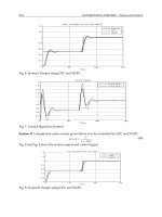
Let us return to the example of the total cost function TC = f(Q) intro-
duced earlier. Consider the hypothetical total cost function in Figure 2.13,
and the corresponding average total cost and marginal cost curves in Figure
2.14.
In Figure 2.13, the numerical value of ATC is the same as a slope of a
ray from the origin to a point on the TC curve corresponding to a given
level of output. The equation of a ray from the origin is TC = bQ, where b
is the slope of the ray from the origin to a point on the TC curve, which is
given as
dA
dx
fx
fx
x
MA=ޢ
()
=
()
=0,or
dA
dx
fx
fx
x
MA<ޢ
()

>
()
<0,or
dA
dx
fx
fx
x
MA>ޢ
()
>
()
>0,or
dA
dx
xf x f x
x
=
¢
()
-
()
2
M
dy
dx
fx==¢
()
A
y

x
fx
x
==
()
yfx=
()
74 introduction to mathematical economics
(2.65)
where the values where Q
1
represents the initial value of output and Q
2
represents the changed level of output. Since the ray passes through
the origin, then the initial values (Q
1
, TC
1
) are (0, 0). Setting TC
2
= TC and
Q
2
= Q, Equation (2.66) reduces to
(2.66)
Of course, the value of b will change as we move along the total cost curve.
This is illustrated in Figure 2.13. MC, of course, is the value of the slope of
the TC curve and may be illustrated diagrammatically in Figure 2.13 as the
slope a line that is tangent to TC at some level of output. By comparing the
value of the slope of the tangent with the slope of the ray from the origin,

we are able to illustrate the relationship between MC and ATC in Figure
2.14.
Note that output at point A in Figure 2.13, the slope of the tangent (MC),
is less than the slope of the ray from the origin (ATC). Thus, at output level
Q
1
, MC is less than ATC. This is illustrated in Figure 2.14. Now let us move
to point B. Note that at Q
2
the slopes of the tangent and the ray are less
than they were at point A. Thus, in Figure 2.14 MC and ATC at Q
2
are less
than at Q
1
.Although both MC and ATC have fallen, the slope of the tangent
(MC) at Q
2
is still less than the slope of the ray (ATC). Thus, since MC <
ATC at Q
2
, then ATC has declined. By analogous reasoning, as we move
from Q
2
to Q
3
, since MC < ATC, then ATC will fall. The reader will note
that point C in the Figure 2.13 is an inflection point. Beyond output level
Q
3

, the slope of the TC curve (MC) begins to increase.Thus, at output level
Q
3
, marginal cost is minimized. Nevertheless, as illustrated in Figure 2.14,
as long as MC < ATC, then ATC will continue to fall.
b ATC
TC
Q
==
b
TC
Q
TC TC
QQ
==
-
-
D
D
21
21
total, average, and marginal relationships 75
TC
TC
Q
0 Q
1
Q
2
Q

3
Q
4
A
B
C
E
Q
5
D
FIGURE 2.13 The total cost curve
and its relationship to marginal and average
total cost.
At output level Q
4
the slopes of the ray and tangent are identical (ATC
= MC). Thus, at Q
4
ATC is neither rising nor falling (i.e., dATC/dQ = 0).
After Q
4
the slope of the tangent not only becomes greater than the slope
of the ray, but the slope of the ray changes direction and starts to increase.
Thus, we see that at output level Q
5
, MC > ATC and ATC are rising. These
relationships are illustrated in Figure 2.14.
The situation depicted in Figure 2.14 illustrates a U-shaped average total
cost curve in which the MC intersects ATC from below. The reader should
visually verify that when MC < ATC, even when MC is rising, ATC is falling.

Moreover, when MC > ATC, then ATC is rising. Finally, when MC = ATC,
then ATC is neither rising nor falling (i.e., ATC is minimized). In some cases,
the average curve is shaped not like U but like a hill: that is, the marginal
curve intersects the average curve from above at its maximum point. An
example of this would be the relationship between the average and mar-
ginal physical products of labor, which will be discussed in detail in Chapter
5.
PROFIT MAXIMIZATION: THE FIRST-ORDER
CONDITION
We are now in a position to use the rules for taking first derivatives to
find the level of output Q that maximizes p, as illustrated in Table 2.3. Con-
sider again the total revenue and total cost functions introduced earlier:
(2.67)
p=- - + -615 9
23
QQQ
p= - = - + - +
()
TR TC Q Q Q Q18 6 33 9
23
TC Q Q Q Q
()
=+ - +633 9
23
TR Q PQ P
()
==; $18
76 introduction to mathematical economics
AT
C

A
TC, MC
Q0 Q
1
Q
2
Q
3
Q
4
MC
Q
5
FIGURE 2.14 The relationship
between average total cost and marginal
cost.
It should be noted in Table 2.3 and Figure 2.11 that profit is maximized
(p=19) at Q = 5. What is more, it should be immediately apparent that if
a smooth curve is fitted to Figure 2.11, the value of the slope at Q = 5 is
zero: that is, the profit function is neither upward sloping nor downward
sloping. Alternatively, at Q = 5, then dp/dQ = 0. These observations imply
that the value of a function will be optimized (maximized or minimized)
where the slope of the function is equal to zero. In the present context, the
first-order condition for profit maximization is dp/dQ = 0, thus
(2.68)
This equation is of the general form:
(2.69)
where a =-8, b = 10 and c =-15. Quadratic equations generally admit to
two solutions, which may be determined using the quadratic formula. The
quadratic formula is given by the expression:

(2.70)
After substituting the values of Equation (2.68) into Equation (2.70) we
get
Referring again to Figure 2.11, we see that the value of p reaches a
minimum and a maximum at output levels of Q = 1 and Q = 5, respectively.
Substituting these values back into the Equation (2.67) yields values of
p=-13 (at Q = 1) and p=19 (at Q = 5). In this example, therefore, the
entrepreneur of the firm would maximize his profits at Q = 5. As this
example illustrates, simply setting the first derivative of the function equal
to zero is not sufficient to ensure that we will achieve a maximum, since a
zero slope is also required for a minimum value as well. Thus, we need to
specify the second-order conditions for a maximum or a minimum value to
be achieved.
Q
2
18 12
6
6
6
1=
-+
-
=
-
-
=
Q
1
2
18 18 4 3 15

23
18 324 180
4
18 12
6
30
6
5
=
-+
()

()
-
()
-
()
=
-+ -
-
=

-
=
-
-
=
x
bb ac
a

12
2
4
2
,
=
-± -
ax bx c
2
0++=
d
dQ
QQ
p
=- + - =318150
2
profit maximization: the first-order condition 77
PROFIT MAXIMIZATION: THE SECOND-ORDER
CONDITION
MAXIMA AND MINIMA
For functions of one independent variable, y = f(x), a second-order con-
dition for f(x) to have a maximum at some value x = x
0
is that together with
dy/dx = f¢(x) = 0, the second derivative (the derivative of the derivative) be
negative, that is,
(2.71)
where f≤(x) is an alternative way to denote the second derivative.
This condition expresses the notion that in the case of a maximum, the
slope of the total function is first positive, zero, and then negative as we

“walk” over the top of the “hill.” Functions that are locally maximum are
said to be “concave downward” in the neighborhood of the maximum value
of the dependent variable. Similarly, the second-order condition for f(x) to
have a minimum at some value x = x
0
, then is
(2.72)
The first-order and second-order conditions for a function with a maxi-
mum or minimum are summarized in Table 2.4.
Consider again the p maximization example, which is also illustrated in
Figure 2.11. Taking the second derivative of the p function yields
At Q
1
= 5,
which is, as we have already seen, a p maximum. At Q
2
= 1,
d
dQ
2
2
6 5 18 30 18 12 0
p
=-
()
+=-+=-<
d
dQ
Q
2

2
618
p
=- +
ddydx
dx
dydx f x
()
==¢¢
()
>
22
0
ddydx
dx
dy
dx
fx
()
==¢¢
()
<
2
2
0
78 introduction to mathematical economics
TABLE 2.4 First-order and second-order conditions for
functions of one independent variable.
Maximum Minimum
First-order condition

Second-order condition
dy
dx
2
2
0>
dy
dx
2
2
0<
dy
dx
=
0
dy
dx
=
0
which is a p minimum.
Problem 2.7. A monopolist’s total revenue and total cost functions
are
a. Determine the output level (Hint: p(Q) = TR(Q) - TC(Q)) that will max-
imize profit p.
b. Determine maximum p.
c. Determine the price per unit at which the p-maximizing output is
sold.
Solution
a. p=TR - TC
= 20Q - 3Q

2
- 2Q
2
= 20Q - 5Q
2
= 20 - 10Q = 0 (i.e., the first-order condition for a profit maximum).
Q = 2 units
=-10 < 0 (i.e., the second-order condition for a profit maximum).
b. p=20(2) - 5(2)
2
= 40 - 20 = $20
c. TR = PQ = 20Q - 3Q
2
= (20 - 3Q)Q
P = 20 - 3Q = 20 - 3(2) = 20 - 6 = $14
Problem 2.8. Another monopolist has the following TR and TC functions:
Find the p-maximizing output level.
Solution
=-12 + 15Q - 3Q
2
= 0 (i.e., the first-order condition for a local
maximum)
Utilizing the quadratic formula:
d
dQ
p
p= -
=-
()
-+ - +

()
=- - + -
TR TC
QQ QQQ QQQ45 05 257 8 212 75
223 23

TC Q Q Q Q
()
=+ - +257 8
23
TR Q Q Q
()
=-45 0 5
2
.
d
dQ
2
2
p
d
dQ
p
TC Q Q
()
= 2
2
TR Q PQ Q Q
()
== -20 3

2
d
dQ
2
2
61 18 6 18 12 0
p
=-
()
+=-+=>
profit maximization: the second-order condition 79
To determine whether these values constitute a minimum or a maximum,
we can substitute the values into the profit function and determine the
minimum and maximum values directly, or we can examine the values of
the second derivatives:
For Q
1
= 4,
(i.e., the second-order condition for a local maximum)
For Q
2
= 1,
(i.e., the second-order condition for a local minimum)
Substituting Q
1
= 4 into the p function yields a maximum profit of
INFLECTION POINTS
What if both the first and second derivatives are equal to zero? That is,
what if f¢(x) = f≤(x) = 0? In this case, we have a stationary point, which
is neither a maximum nor a minimum. That is, stationary values for which

f¢(x) = 0 need not be a relative extremum (maximum or minimum). Sta-
tionary values at x
0
that are neither relative maxima nor minima are illus-
trated in Figures 2.15 and 2.16.
To determine whether the stationary value at x
0
is the situation depicted
in Figure 2.15 or Figure 2.16, it is necessary to examine the third derivative:
d(d
2
y/dx
2
)/dx = d
3
y/dx
3
= f¢¢¢ (x). The value of the third derivative for the
p*.=- -
()
+
()
-= + -=2 12 4 7 5 4 2 48 120 64 6
2
3
Q
d
dQ
2
2

6 1 15 6 15 9 0
p
=-
()
+=-+=>
d
dQ
2
2
6 4 15 24 15 9 0
p
=-
()
+=-+=-<
d
dQ
Q
2
2
615
p
=- +
Q
2
15 9
6
6
6
1=
-+

-
=
-
-
=
Q
1
15 9
6
24
6
4=

-
=
-
-
=
Q
12
2
15 15 4 3 12
23
15 81
6
15 9
6
,
=
-±

()
-
()
-
()
=
-±
-
=
-±
-
80 introduction to mathematical economics
situation depicted in Figure 2.15 is d
3
y/dx
3
= f¢¢¢(x) > 0.The value of the third
derivative for the situation depicted in Figure 2.16 is d
3
y/dx
3
= f¢¢¢(x) < 0.
PARTIAL DERIVATIVES AND MULTIVARIATE
OPTIMIZATION: THE FIRST-ORDER
CONDITION
Most economic relations involve more than one independent (explana-
tory) variable. For example, consider the following sales (Q) function of a
firm that depends on the price of the product (P) and levels of advertising
expenditures (A):
(2.73)

To determine the marginal effect of each independent variable, we take
the first derivative of the function with respect to each variable separately,
QfPA=
()
,
the first-order condition 81
f(x)
x
0
0
x
FIGURE 2.15 Inflection point: a
stationary value at x
0
that is neither a
maximum nor a minimum.
f(x)
x
0
0
x
FIGURE 2.16 Inflection point: a
stationary value at x
0
that is neither a
maximum nor a minimum.
treating the remaining variables as constants. This process, known as taking
partial derivatives, is denoted by replacing d with ∂.
Example
Consider the following explicit relationship:

(2.74)
(where A is in thousands of dollars). Taking first partial derivatives with respect to
P and A yields
(2.75)
(2.76)
To determine the values of the independent variables that maximize the
objective function, we simply set the first partial derivatives equal to zero
and solve the resulting equations simultaneously.
Example
To determine the values of P and A that maximize the firm’s total sales, Q, set the
first partial derivatives in Equations (2.69) and (2.70) equal to zero.
(2.77)
(2.78)
Equations (2.77) and (2.78) are the first-order conditions for a maximum. Solving
these two linear equations simultaneously in two unknowns yields (in thousands of
dollars).
Substituting these results back into Equation (2.74) yields the optimal value of Q.
PARTIAL DERIVATIVES AND MULTIVARIATE
OPTIMIZATION: THE SECOND-ORDER
CONDITION
8
Unfortunately, a general discussion of the second-order conditions for
multivariate optimization is beyond the scope of this book. It will be suffi-
cient within the present context, however, to examine the second-order con-
ditions for a maximum and a minimum in the case of two independent
variables. Consider the following function:
Q*. . . .
$, .
=
()

-
()
-
()()
-
()
+
()
=
80 16 52 2 16 52 16 52 13 92 3 13 92 100 13 92
1 356 52
22
A = $.13 92
P = $.16 52
+ =PA6 100 0
80 4 0 =PA
∂
∂
Q
A
PA=- - +6 100
∂
∂
Q
P
PA=- -80 4
QfPA P P PA A A=
()
= +,802 3100
22

82 introduction to mathematical economics
8
For a more complete discussion of the second-order conditions for the multivariate case,
see Silberberg (1990), Chapter 4.
(2.79)
As discussed earlier, the first-order conditions for a maximum or a
minimum are given by
(2.80a)
(2.80b)
The second-order conditions for a maximum are given by
(2.81a)
(2.81b)
(2.81c)
The second-order conditions for a minimum are given by:
(2.82a)
(2.82b)
(2.82c)
Example
Consider once again our sales maximization problem.The appropriate second-order
conditions are given by:
(2.83a)
(2.83b)
(2.83c)
The second-order conditions for sales maximization are satisfied.
9
The first- and
second-order conditions for sales maximization are illustrated in Figure 2.17.
ff f
PP AA PA
-=-

()
-
()

()
=+>
22
4 6 1 2410
f
AA
=- <60
f
PP
=- <40
∂
∂
∂
∂
∂
∂∂
2
1
2
2
2
2
2
12
2
11 22 12

2
0
y
x
y
x
y
xx
ff f
Ê
Ë
ˆ
¯
Ê
Ë
ˆ
¯
-
Ê
Ë
ˆ
¯
=->
∂
∂
2
2
2
22
0

y
x
f=>
∂
∂
2
1
2
11
0
y
x
f=>
∂
∂
∂
∂
∂
∂∂
2
1
2
2
2
2
2
12
2
11 22 12
2

0
y
x
y
x
y
xx
ff f
Ê
Ë
ˆ
¯
Ê
Ë
ˆ
¯
-
Ê
Ë
ˆ
¯
=->
∂
∂
2
2
2
12
0
y

x
f=<
∂
∂
2
1
2
11
0
y
x
f=<
∂
∂
y
x
f
2
2
0==
∂
∂
y
x
f
1
1
0==
yfxx=
()

12
,
the second-order condition 83
9
By Young’s theorem
That is, the same “cross partial” derivative results regardless of the order in which the vari-
ables are differentiated. For a more complete discussion of Young’s theorem, see Silberberg
(1990), Chapter 3. According to Silberberg, the reference is to W. H. Young who published a
ff
xy yx
=
CONSTRAINED OPTIMIZATION
Unfortunately, most decision problems managers faced are not of the
unconstrained variety just discussed.The manager often is required to max-
imize some objective function subject to one or more side constraints. A
production manager, for example, may be required to maximize the total
output of a given commodity subject to a given budget constraint and fixed
prices of factors of production. Alternatively, the manager might be
required to minimize the total costs of producing some specified level of
output. The cost minimization problem might be written as:
Maximize (or minimize): (2.84a)
Subject to: (2.84b)
Example
The total cost function of a firm that produces its product on two assembly lines is
given as
The problem facing the firm is to determine the least-cost combination of output
on assembly lines x and y subject to the side condition that total output equal 20
units. This problem may be formally written as
Minimize:
Subject to:

xy+=20
TC x y x y xy,
()
=+-36
22
TC x y x y xy,
()
=+-36
22
kgxx=
()
12
,
yfxx=
()
12
,
84 introduction to mathematical economics
formal proof of this theorem in 1909 using the concept of the limit (see, e.g., Cambridge Tract
No. 11, The Fundamental Theorems of the Differential Calculus, Cambridge University Press,
reprinted in 1971 by Hafner Press). According to Silberberg, the result was first published
by Euler in 1734 (“De infinitis curvis eiusdem generis ,” Commentatio 44 Indicis
Enestroemiani).
∂Q/∂ A=0
∂Q/∂
P=0$1,356.52
$13.92
$16.52
P
P*

0
A
A*
Q
FIGURE 2.17 A global maximum.
SOLUTION METHODS TO CONSTRAINED
OPTIMIZATION PROBLEMS
There are generally two methods of solving constrained optimization
problems:
1. The substitution method
2. The Lagrange multiplier method
SUBSTITUTION METHOD
The substitution method involves first solving the constraint, say for x,
and substituting the result into the original objective function. Consider,
again, the foregoing example.
(2.85)
Substituting into the objective function yields
(2.86)
(2.87)
In other words, this problem reduces to one of solving for one decision
variable, y, and inserting the solution into the objective function.Taking the
first derivative of the objective function with respect to y and setting the
result equal to zero, we get
(2.88)
Note also that the second-order condition for total cost minimization is
also satisfied:
(2.89)
Substituting y = 7 into the constraint yields
Finally, substituting the values of x and y into the original TC function
yields:

x = 13
x +=720
dTC
dy
2
2
20 0=>
y = 7
20 140y =
dTC
dy
y=- + =140 20 0
TC y y=-+1200 140 10
2
TC f g y F y y y y y
yy y yy
=
()
[]
=
()
=-
()
+
()
=-+
()
+- -
()
30 20 6 20

3 400 40 6 20
2
2
22 2
xgy y=
()
=-20
solution methods to constrained optimization problems 85
LAGRANGE MULTIPLIER METHOD
Sometimes the substitution method may not be feasible because of more
than one side constraint, or because the objective function or side con-
straints are too complex for efficient solution. Here, the Lagrange multiplier
method can be used, which directly combines the objective function with
the side constraint(s).
The first step in applying the Lagrange multiplier technique is to first
bring all terms to the right side of the equation.
10
With this, we can now form a new objective function called the Lagrange
function, which will be used in subsequent chapters to find solution values
to constrained optimization:
(2.90)
Note that this expression is equal to the original objective function, since
all we have done is add zero to it. That is, ᏸ always equals f for values of x
and y that satisfy g. To solve for optimal values of x and y, we now take the
first partials of this more complicated expression with respect to three
unknowns—x, y, and l. The first-order conditions therefore become:
(2.91a)
(2.91b)
(2.91c)
Note that Equation (2.91c) is, conveniently, our original constraint. Since

the first-order conditions given constitute three linear equations in three
unknowns, this system of equations may be solved simultaneously.The solu-
tion values are
xy===-13 17 71;;l
∂
∂l
l
ᏸ
ᏸ== =12 0xy
∂
∂
l
ᏸ
ᏸ
y
yx
y
== =12 0
∂
∂
l
ᏸ
ᏸ
x
xy
x
== =60
ᏸ xy fxy gxy
xyxy xy
,, ,

()
=
()
+
()
=+-+
()
l
l36 20
22
20 0 =xy
TC =
()
+
()
-
()()
=+-=3 13 6 7 13 7 507 294 91 710
22
86 introduction to mathematical economics
10
Actually, it does not really matter whether the terms are brought to the right- or to the
left-hand side of the equation, although it will affect the interpretation of the value of the
Lagrange multiplier, l. In other words, it is of no consequence whether one writes ᏸ = f +lg
or ᏸ = f -lg, since one’s choice merely changes the sign of the Lagrangian multiplier.