Managerial economics theory and practice phần 10 pot

Although it is not possible to estimate the probabilities of all possible
outcomes, the Hurwicz decision criterion is an attempt to incorporate the
decision maker’s attitude toward risk into the Wald decision criterion by
creating a decision index for each strategy.This index is a weighted average
of the maximum and minimum payoff from each strategy. These weights
are called coefficients of optimism.The equation for estimating the Hurwicz
decision index for each strategy is
(14.18)
where D
i
is the decision index, M
i
is the maximum payoff from each strat-
egy, m
i
is the minimum payoff from each strategy, and a is the coefficient
of optimism. The optimal strategy using the Hurwicz decision criterion has
the highest value for D
i
.
Definition:The Hurwicz decision criterion is a decision-making approach
in the presence of complete ignorance in which the optimal strategy is
selected based on a decision index calculated from a weighted average of
the maximum and minimum payoff of each strategy.The weights, which are
called coefficients of optimism, are measures of the decision maker’s atti-
tude toward risk.
The value of the coefficient of optimism, which ranges in value from 0
to 1, represents management’s subjective attitude toward risk. When a=0,
the decision maker is completely pessimistic about the outcomes. When a
= 1, the decision maker is completely optimistic about the outcomes. Figure
14.19 summarizes the estimated values of the Hurwicz indices for selected

values of a between 0 and 1. Consider, for example, a relatively pessimistic
manager with a coefficient of optimism of a=0.3. From the maximum and
minimum payoffs summarized in Figure 14.12, the Hurwicz decision index
for a “raise price” strategy is
The reader should verify that when a=0 the optimal strategy under the
Hurwicz decision is identical to the optimal strategy that would be selected
by using the extremely pessimistic Wald (maximin) decision criterion.
Moreover, when a=1, the optimal strategy under the Hurwicz decision cri-
terion is identical to the optimal strategy obtained by using the maximax
decision criterion. Figure 14.19 identifies the optimal strategies from the
highest values for D
i
with an asterisk. For values for a<0.5, the optimal
(risk-averse) decision criterion is the “lower price” strategy. For values of
a>0.5, the optimal (risk-loving) decision criterion is a “raise price” strat-
egy. When a=0.5, the decision maker is indifferent to the different pricing
strategies.
The Hurwicz decision criterion is superior to the Wald decision criterion
because it forces managers to confront their attitudes toward risk. More-
DM m
ii i
=+-
()
=
()
+-
()
-
()
=

aa1
0 3 25 1 0 3 10 0 5
DM m
ii i
=+-
()
aa1
662 Risk and Uncertainty
over, it forces managers to be consistent when they are considering the
relative merits of alternative strategies. Of course, one drawback to this
approach is the possible negative impact on company earnings should
management’s sense of optimism prove to be misplaced. Of course, this
criticism might be leveled at any decision criterion that involves the sub-
jective determination of probabilistic outcomes. In spite of this, the Hurwicz
decision criterion does represent a conceptual improvement over the some-
what arbitrary Wald decision criterion.
SAVAGE DECISION CRITERION
The Savage decision criterion, which is sometimes referred to as the
minimax regret criterion, is based on the opportunity cost (or regret) of
selecting an incorrect strategy. In this instance, opportunity costs are mea-
sured as the absolute difference between the payoff for each strategy and
the strategy that yields the highest payoff from each state of nature. Once
these opportunity costs have been estimated, the manager will select the
strategy that results in the minimum of all maximum opportunity costs.
Definition: The Savage decision criterion is used to determine the
strategy that results in the minimum of all maximum opportunity costs
associated with the selection of an incorrect strategy.
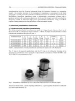
Figure 14.20 illustrates the calculations of the opportunity costs for the
payoffs summarized in Figure 14.12. For example, the maximum possible
payoff during an economic expansion is 25 for a “raise price” strategy. The

absolute difference between the maximum payoff and the payoffs from
each strategy during an economic expansion are calculated and summarized
in each cell of the matrix. Figure 14.20 summarizes the maximum regret
(opportunity cost) from each strategy. The minimum of these maximum
opportunity costs, which is identified with an asterisk, is the strategy that
will be selected by means of the Savage decision criterion.
Neither overly optimistic nor overly pessimistic, the Savage decision
criterion is most appropriate when management is interested in earning a
satisfactory rate of return with moderate levels of risk over the long term.
Thus, the Savage decision criterion may be more appropriate for long-term
capital investment projects.
Decision Making Under Uncertainty with Complete Ignorance 663
␣ =
0.0 0.1 0.2 0.3 0.4 0.5 0.6 0.7 0.8 0.9 1.0
Ϫ
10
Ϫ
6.5 !3 0.5 4 7.5* 11* 14.5* 18* 21.5* 25*
Ϫ
5
Ϫ
2.5 0 2.5 5 7.5* 10 12.5 15 17.5 20
0* 1.5* 3* 4.5* 6* 7.5* 9 10.5 12 13.5
15
Raise price
No change
Lower price
FIGURE 14.19 Estimated Hurwicz D values for selected values of a, the coefficient of
optimism.
MARKET UNCERTAINTY AND INSURANCE

Markets operate best when all parties have equal access to all informa-
tion regarding the potential costs and benefits associated with an exchange
of goods or services. When this condition is not satisfied, then uncertainty
exists and either the buyer or the seller may be harmed, which will result
in an inefficient allocation of resources. In this section, we will examine
some of the problems that arise in the presence of market uncertainty.
ASYMMETRIC INFORMATION
For markets to operate efficiently, both the buyer and the seller must
have complete and accurate information about the quantity, quality, and
price of the good or service being exchanged. When uncertainty is present,
market participants can, and often do, make mistakes. An important cause
of market uncertainty is asymmetric information. Asymmetric information
exists when some market participants have more and better information
than others about the goods and services being exchanged. An extreme
example of the problems that might arise in the presence of asymmetric
information is fraud. The reader will recall from Chapter 13 the discussion
of the “snake oil” salesman, who traveled from frontier town to frontier
town in the American West selling bottles of elixirs promising everything
from a cure for toothaches to a remedy for baldness. Of course, these claims
were bogus, but by the time customers realized that they had been “had”
the snake oil salesman was long gone. Had the customer known that the
elixir was worthless, the transaction would never have taken place.
In the extreme case, the knowledge that, some market participants had
improperly exploited their access to privileged information could result in
a complete breakdown of the market. In insider trading, for example, some
market participants have access to classified information about a firm whose
shares are publicly traded. Thus an executive who discovers that senior
management of his firm plans to merge with a competitor, which will result
in an increase in the firm’s stock price, might act on this information by
buying shares of stock in his own company. This person is guilty of insider

664 Risk and Uncertainty
Raise price
No change
Lower price
Economy
Expansion Stability Contraction
Maximum
regret
͉25
Ϫ25͉ = 0 ͉15 Ϫ20͉ = 5 ͉Ϫ10 Ϫ5͉ = 15 15
Strategy
͉15 Ϫ25͉ = 10 ͉ 20 Ϫ20͉ = 0 ͉Ϫ5 Ϫ5͉ = 10 10*
͉15
Ϫ25͉ = 10 ͉ 0 Ϫ20͉ = 20 ͉5Ϫ5͉ = 0 20
FIGURE 14.20 Savage regret matrix.
trading. When insider trading is pervasive, rational investors who are not
privy to privileged information may choose not to participate at all, rather
than to put themselves at risk of buying or selling shares at the wrong
price.
The uncertainty arising from asymmetric information affects managerial
decisions as well. The reader will recall from Chapter 7, for example, that a
profit-maximizing competitive firm will hire additional workers as long as
the additional revenue generated from sale of the increased output (the
marginal revenue product of labor) is greater than the wage rate. The mar-
ginal revenue product of labor is defined as the price of the product times
the marginal product of labor, P ¥ MP
L
. But how is the manager to know
the potential productivity of a prospective job applicant? This is a classic
example of asymmetric information. The prospective job applicant has

much better information than the manager about his or her skills, capabil-
ities, integrity, and attitude toward work. Since the potential cost to the firm
of hiring an unproductive worker may be very high, managers will take
whatever reasonable measures are necessary to rectify this asymmetry. This
is why firms require job applicants to submit résumés, college transcripts,
letters of recommendations, and so on. The firm’s human resources officer
may require job applicants to be interviewed by responsible professionals
within the firm. Firms may also conduct background and credit checks,
require applicants to sit for examinations to evaluate job skills, mandate
probationary periods prior to full employment, and so forth.
ADVERSE SELECTION
The problem of adverse selection arises whenever there is asymmetric
information.The classic example of adverse selection is the used-car market
(Akerlof, 1970). A person with a used car to sell has the option of selling
the vehicle to a used-car dealer or selling it privately. For simplicity, assume
that all the used cars for sale are similar in every respect (age, features, etc.)
except that half are “lemons” (bad cars) and the others are plums (good
cars). Finally, suppose that potential buyers are willing to pay $5,000 for a
plum and only $1,000 for a lemon.
Potential buyers have no way of distinguishing between lemons and
plums. Since there is a fifty-fifty chance of getting a lemon, the expected
market price of the used car is $3,000. Since only the sellers know whether
their cars are lemons, there is a problem of asymmetric information. The
seller has the option of selling to a used-car dealer or selling privately. If a
lemon is sold to the used-car dealer for $3,000, then the seller will extract
$2,000 at the expense of the buyer, while if a plum sells for $3,000, then the
buyer will extract $2,000 at the expense of the seller. Thus, it is in the best
interest of lemon owners to sell to used-car dealers, while it is in the best
interest of plum owners to sell privately.
Market Uncertainty and Insurance 665

Buyers of used cars have the choice of buying from a used-car dealer or
buying directly from an owner. Of course, buyers come to realize that prob-
ability of buying a lemon from a used-car dealer is greater than from buying
from the owner directly. Thus, the used-car dealer price will fall. This will
further exacerbate matters, since it will create an even greater incentive for
plum owners to avoid the used-car market and sell privately. In the end,
only lemons will be available from used-car dealers. In this case, the lemons
drive the plums out of the market. This is an example of adverse selection.
Here, the market has adversely selected the product of inferior quality
because of the presence of asymmetric information.
Definition: In the presence of asymmetric information, adverse selection
refers to the process in which goods, services, and individuals with eco-
nomically undesirable characteristics tend to drive out of the market goods,
services, and individuals with economically desirable characteristics.
The problem of adverse selection is particularly problematic in the
market for insurance. As discussed earlier, risk-averse individuals purchase
insurance to eliminate the risk of catastrophic financial loss in exchange for
premium payments that are small relative to the potential loss.The problem
confronting an insurance company is that it is difficult to distinguish high-
risk from low-risk individuals. One possible solution would be for insurance
companies to charge an insurance premium that is a weighted average of
the premiums charged to individuals falling into different risk categories.
In this case, high-risk individuals will purchase insurance policies while
low-risk individuals will not. As a result, the insurance company will have
to revise upward its insurance premium just to break even.
As an illustration of adverse selection in the insurance market, consider
a firm that sells automobile collision insurance to residents of a particular
area.The insurance company has identified two, equal-sized groups of high-
risk and low-risk individuals. The insurance company has decided that the
probability of an automobile accident is p = 0.1 for a member of the high-

risk group and only p = 0.01 for a member of the low-risk group. If there
are 100 people in each group, this is tantamount to an average of 10 auto-
mobile accidents per year for the high-risk group compared with one for
the low-risk group. Suppose that the average repair bill per automobile acci-
dent is $1,000. If the insurance premium charged is the expected average
repair bill loss, then the firm should charge the high-risk group 0.1($1,000)
= $100 per year and the low-risk group 0.01($1,000) = $10 per year. If it is
not possible for the insurance company to identify the members of each
group, then the insurance company could decide to charge a premium based
on the average risk, that is, 0.5($100) + 0.5($10) = $55.
The situation just described gives rise to the problem of adverse selec-
tion. If the insurance company charges a premium of $55, then some
members of the low-risk group will opt not to purchase insurance. If 50
members of the low-risk group decide to withdraw from the insurance
666 Risk and Uncertainty
market, then the total pool of individuals buying insurance falls from 200
to 150. As a result, the premium charged will increase to 0.67($100) +
0.33($10) = $70.3. Of course, some of the remaining individuals in the low-
risk group will find that this premium is too high and will, in turn, withdraw
from the insurance market. This process will continue until, in the end, only
the most risk-averse individuals continue to buy insurance or, which is more
likely, only members of the high-risk group remain.
FAIR-ODDS LINE
It is possible to analyze the problem of adverse selection by recasting
individuals’ attitudes toward risk within the framework of state-dependent
indifference curves.
1
Consider again the situation in which an individual
is offered a fair gamble on the flip of a coin. Suppose that the individual
has $1,000. The person can bet all or part of this amount on the flip of a

coin. If the coin comes up “heads,” then the individual wins $1 for every $1
wagered. If the coin comes up “tails,” then the individual loses $1 for every
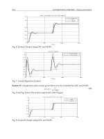
$1 wagered. Figure 14.21 illustrates the results of alternative wagers from
this fair gamble. The horizontal axis represents the individual’s money
holdings if the coin comes up tails, while the vertical axis represents the
individual’s money holdings if the coin comes up heads. In a broader sense,
the horizontal and vertical axes of Figure 14.21 may be thought of as the
outcomes of two probabilistic states of nature. Point C in Figure 14.21
identifies the individual’s money holdings on a decision not to bet. That is,
regardless of the results of the flip of the coin, the individual will still have
a cash “endowment” of $1,000, since no amount was placed at risk.
Market Uncertainty and Insurance 667
1
For a detailed discussion of indifference curves see, for example, Walter Nicholson,
Microeconomic Theory: Basic Principles and Extensions, 6
th
ed. (Font Worth: The Dryden
Press, 1995), Chapter 3.
0 Tails
Heads
A (0, 2000)
B (500, 1500)
C (1000, 1000)
D (2000, 0)
1,000
1,000
1,500
500
FIGURE 14.21 Fair-odds line for
different states of nature.

Suppose that the individual decides to wager $500 on the flip of the coin.
If the coin comes up heads, then the individual wins $500. If the coin comes
up tails, then the individual loses $500. Point B in Figure 14.21 illustrates
the possible outcomes of this bet. If the individual loses the wager, then his
or her endowment is reduced to $500. On the other hand, if the individual
wins the wager, his or her endowment is increased to $1,500. This combi-
nation of outcomes is identified in the parentheses at point B.Alternatively,
if the individual wagers the entire $1,000, then the possible combination of
outcomes corresponds to point A, where the individual is left penniless if
the coin comes up tail but has an endowment of $2,000 if the coin comes
up heads. What about the points in Figure 14.21 below C, such as point D?
Points below point C represent a reversal of the terms of the wager (i.e.,
tails wins and heads loses).
The situation depicted in Figure 14.21 is analogous to the budget con-
straint introduced in Chapter 7 in that the endowments define the individ-
ual’s consumption possibilities. Figure 14.21 is referred to as the individual’s
fair-odds line. In general, whenever the expected value of a wager is zero,
then the gamble is said to be actuarially fair. A gamble is said to be fair if
its expected value is zero. In the foregoing example, if the individual decides
not to wager any amount, he or she is left with the initial endowment of
$1,000. If the individual decides to wager some amount, the expected value
of the bet is zero, in which case the expected value of the endowment is still
$1,000.
The fair-odds line in Figure 14.21 is summarized in Equation (14.19),
which represents an actually fair gamble where p is the probability of a
monetary gain if the individual wins the bet and (1 - p) is the probability
of a monetary loss if the individual loses the bet.
(14.19)
The slope of the fair-odds line is given as the monetary gain divided by
the monetary loss from a fair gamble. Suppose, for example, that the indi-

vidual places a wager of $500. If the individual wins the bet, his or her
endowment will increase to $1,500 (i.e., the amount of the gain is W = $500).
On the other hand, if the individual loses the bet, his or her endowment is
reduced to $500 (i.e., L =-$500). This is illustrated as a move from point C
to point B in Figure 14.21. Solving Equation (14.19), we obtain
(14.20)
The reader should verify that the budget constraint depicted in Figure
14.21 had a slope of -1. The reader should also verify that, in general, an
increase in the probability of winning means that for the gamble to remain
fair, the amount of the win will have to decrease. For example, when p =
0.5, then W/L =-(1 - 0.5)/0.5 =-1. If the probability of winning increases
W
L
p
p
=
-1
pW p L+-
()
=10
668 Risk and Uncertainty
to p = 0.75, then W/L =-(1 - 0.75)/0.75 =-0.25/0.75 =-0.33. Similarly, if the
probability of losing increases, the amount of the win will have to increase
for the gamble to remain fair.These three situations are illustrated in Figure
14.22.
STATE PREFERENCES
The indifference curve framework can also be used to identify an indi-
vidual’s attitudes toward risk. In this case, however, the two goods that are
normally identified along the horizontal and vertical axes are replaced with
different combinations of state-dependent consumption levels that yield

equal levels of utility. The shapes of these indifference curves reflect the
individual’s behavior when confronted with risky situations.
In Figure 14.22, which illustrates the case of an individual with risk-
averse preferences, S
1
and S
0
represent two different states of nature. It will
be recalled that an individual with risk-averse preferences will never accept
a fair gamble with an expected value equal to zero. This is because a risk-
averse individual will always prefer a certain sum to an uncertain sum with
the same expected value. Thus, the indifference curves of an individual with
risk-averse preferences are convex with respect to the origin.
The individual described in Figure 14.22 will prefer a consumption level
corresponding to point B to any other point on the fair-odds line. Con-
sumption levels that correspond to points A and C are found on an indif-
ference curve that is closer to the origin, which yields a lower level of utility.
The point of tangency between the fair-odds line and the indifference curve
I
0
at point B represents the highest level of utility that this individual can
attain with a given endowment. At point B the slope of the indifference
curve is -(1 - p)/p. Line 0D, which represents the locus of all such fair-odds
tangency points at fair odds, is called the certainty line, which is analytically
Market Uncertainty and Insurance 669
0
S
1
S
0

I
0
I
1
I
2
I
Ϫ
1
45Њ
A
D
B
C
Certainty line
FIGURE 14.22 Indifference map of
risk-averse preferences.
equivalent to the income consumption curve in utility theory and the expan-
sion path in production theory. The certainty line represents equal con-
sumption in either state of nature.
The choices confronting a person with risk-neutral preferences are illus-
trated in Figure 14.23. Points A, B, and C all yield the same level of utility,
since the indifference curve I
0
corresponds to the fair-odds line. A risk-
neutral individual is indifferent between a certain sum and an uncertain
sum with the same expected value. Finally Figure 14.24 illustrates the case
of a risk-loving individual.A risk lover will always accept a fair gamble with
an expected value equal to zero. Risk lovers have indifference curves that
are concave with respect to the origin. Accepting a fair gamble will move

the individual away from point B and result in a higher level of utility. In
fact, concave indifference curves will invariably result in a corner solution,
such as points A and C, in which the individual will gamble the total amount
of his or her endowment.
670 Risk and Uncertainty
0
S
1
S
0
I
0
I
1
I
2
I
Ϫ1
45Њ
C
A
B
C
FIGURE 14.23 Indifference map of
risk-neutral preferences.
0
S
1
S
0

I
0
I
1
I
2
I
Ϫ
1
45Њ
A
D
B
C
FIGURE 14.24 Indifference map of
risk-loving preferences.
INSURANCE PREMIUMS
The state preferences model just presented can be used to analyze the
demand for insurance. We will initially assume that insurance is provided
at zero administrative cost. We will also assume that insurance is offered at
actuarially fair terms. In the event of an adverse state of nature, the insur-
ance company agrees to pay out the full amount of the loss, while in a favor-
able state of nature the insurance company pays nothing. The insurance
premium is equal to the expected value of the payout, that is,
(14.21)
where (1 - p) is the probability of an adverse state of nature, such as the
financial loss arising from an accident (L), and p is the probability of a
favorable state of nature. In our example of automobile collision insurance,
if the insurance policy provides $1,000 annual coverage and the probabil-
ity of an automobile is 10%, then an actuarially fair premium is $100 per

year. For each additional $100 of coverage the additional premium will
be $10. Figure 14.25 illustrates the situation of an individual buying fair
insurance.
In Figure 14.25 the individual’s endowment is at point A. Suppose that
the individual wishes to equalize his or her consumption in either state of
nature. This will involve moving along the fair-odds line from point A to
point B on the full insurance line 0D. This will involve the payment of an
insurance premium AC in exchange for an insurance payout of CB should
the adverse event occur. In general, risk-averse individuals will purchase
full insurance offered at fair odds. But what if insurance is offered at unfair
odds? This situation is depicted in Figure 14.26.
Thus far we have assumed that insurance companies operate at zero cost.
This assumption allowed us to assume that insurance companies are able
to provide insurance at actuarially fair terms. This assumption is obviously
PpL=
Market Uncertainty and Insurance 671
0
S
1
S
0
I
0
͕
Premium
Payout
D
B
C
A

FIGURE 14.25 Full insurance at fair
odds.
unrealistic, since insurance companies are analytically subject to the same
long-run and short-run production considerations faced by any other firm.
Thus, since the provision of insurance, or any other good or service, is not
free, we must modify our analysis to recognize that the premium charged
is not equal to the expected payout. When insurance is not provided at
fair odds, the fair-odds line will pivot in a clockwise direction around the
individual’s initial endowment. In Figure 14.26, this is illustrated by the
individual’s new budget line that passes through points A and E.
Inspection of Figure 14.26 reveals that when insurance is not provided
at actuarially fair terms, the individual will purchase partial insurance CB
- EB for the same insurance premium AC. In other words, when insurance
is not provided at actuarially fair terms, a risk-averse individual will
nonetheless purchase partial coverage even though the premium payments
are greater than the expected loss. It is evident from Figure 14.26 that insur-
ance provided at unfair odds will move the individual’s consumption level
in either state of nature to a lower indifference curve than would be the
case if insurance were provided at fair odds. As before, in equilibrium the
individual’s marginal rate of substitution between the state-dependent con-
sumption levels is equal to the slope of the fair-odds (budget) constraint,
although consumption levels will obviously be less than in a favorable state
of nature.
We are now in a position to formally analyze the problem of adverse
selection arising from asymmetric information. Recall from the automobile
collision insurance example that the problem of adverse selection arises
when the insurance company is unable to distinguish individuals belonging
to the high- and low-risk groups. In terms of the state preference model,
Figure 14.27 illustrates the fair-odds lines of the high-risk group, the low-
risk group, and the average market risk.

In Figure 14.27, the fair-odds lines of the high- and low-risk groups are
F
H
and F
L
, respectively.The average-market fair-odds line is F
M
. Figure 14.27
672 Risk and Uncertainty
0
S
1
S
0
I
0
EC
A
B
D
FIGURE 14.26 Partial insurance at
unfair odds.
assumes that both the high- and low-risk groups have the same initial
endowment, with is indicated at point B. The different risks associated
with each group are reflected in the slopes of the fair-odds lines, that is,
[-(1 - p
H
)/p
H
] < [-(1 - p

L
)/p
L
]. This is because the probability that an in-
dividual in the high-risk group will have an accident (1 - p
H
) is greater
than the probability that an individual in the low-risk group will have an
accident (1 - p
L
).
The different risks faced by individuals in both groups are also reflected
in the slopes of the indifference curves. Figure 14.28 illustrates the indif-
ference curves for the high- and low-risk groups. Individuals belonging to
the low-risk group are less likely to make a claim under an insurance policy
than individuals belonging to the high-risk group. Thus, low-risk individu-
als will require greater compensation for a given reduction in consumption
in a favorable state of nature. In Figure 14.28, low-risk individuals making
a claim will require an additional amount AE in state of nature S
0
, while
high-risk individuals will require AC < AE. Thus, the indifference curve for
the low-risk individual (I
L
) is flatter than the indifference curve for the high-
risk group (I
H
).
The problem of adverse selection is illustrated in Figure 14.29. Note that
the slope of the low-risk individual’s indifference curve is flatter than the

market-average fair-odds line, F
M
, at the initial endowment point B.In
exchange for a sure amount in a favorable state of nature, AB, the individ-
ual is able to obtain only AC coverage in an adverse state of nature. But,
to be as well off as at point B, the low-risk individual would require an addi-
tional amount CE in an adverse state of nature. Thus, the low-risk individ-
ual would be better off with no insurance at all.
In general, adverse selection is more likely to be a problem when the
market consists of a high proportion of high-risk individuals, which has the
effect of moving the average-market fair-odds line closer to the fair-odds
Market Uncertainty and Insurance 673
0
S
1
S
0
B
F
H
F
L
F
M
FIGURE 14.27 High-risk, low-risk, and
average-market fair-odds lines.
line for the high-risk group (F
H
) in Figure 14.27. Adverse selection is also
more likely to be a problem if there is a large gap in the perceptions toward

risk of the high- and low-risk groups. Adverse selection will be less a prob-
lematic if some individuals are extremely risk averse. In practice, it is
common for insurance companies to differentiate candidates for insurance
to capture different attitudes toward risk.Thus, differential premiums based
on age, sex, occupation, lifestyle, and domicile are a commonly found in the
insurance industry.
MORAL HAZARD
Another problem that arises in the presence of asymmetric information
is the problem of moral hazard. We saw earlier that risk-averse individuals
will purchase insurance to protect themselves against catastrophic financial
674 Risk and Uncertainty
0
S
1
S
0
B
I
H
I
L
E
CA
FIGURE 14.28 The indifference curve
of a low-risk individual is flatter than the
indifference curve of a high-risk individual.
0
S
1
S

0
D
B
CAE
F
M
I
L
FIGURE 14.29 Adverse selection:
low-risk individuals choose not to purchase
insurance.
losses. Of course, the probability that such catastrophic losses will occur is
inversely related to individual efforts to avoid such losses. For example, the
probability of having an automobile accident depends on how carefully one
drives. Other things being equal, individuals tend to be more careful behind
the wheel if they are not insured than when they are fully insured. The
reason for this is that the insured knows that he or she will be fully com-
pensated for damages incurred as a result of an accident. If an insured indi-
vidual has a reduced incentive to be careful, a moral hazard is said to exist.
Other examples of moral hazard include individuals who lead less-than-
healthy lifestyles after obtaining health insurance, or doctors who are less
than conscientious about administering medical care after obtaining
medical malpractice insurance.
Definition: A moral hazard exists when insurance coverage causes an
individual to behave in such a way that changes the probability of incur-
ring a loss.
In general, a moral hazard exists when an individual can determine the
probability of an undesirable outcome. To see this, consider the case of an
insurance company that has estimated that the probability p that an auto-
mobile will be stolen. Ignoring administrative costs, the insurance company

will provide coverage against automobile theft for the premium payment P
in Equation (14.21). Now, suppose that an insured individual can determine
the probability that his or her car will be stolen. Suppose, for example, that
the insured is able to set p = 1. In this case, the insured individual is effec-
tively attempting to use the insurance policy to obtain the price of a new
car. Of course, if the insurance company knows this, automobile theft insur-
ance will not be offered. In this case, a moral hazard exists because the
insurance company does not, indeed cannot, know the probability that the
insured will submit a claim.
The problem of moral hazard may be represented diagrammatically by
means of the state preferences model. Figure 14.30 illustrates the amount
of care that an individual exercises to avoid the probability of an adverse
state of nature. The flatter the indifference curve, the greater the care
an individual takes to avoid a loss. The indifference curves in Figure 14.30
associated with low and high probabilities of an adverse state of nature are
identified as I
L
and I
H
, respectively. To understand why this is the case, we
can ask ourselves the following question: How much will an individual be
willing to sacrifice in an adverse state of nature to obtain a given amount
in a favorable state of nature?
The answer to this question depends on how likely it is that the individ-
ual will experience the adverse state of nature, which, of course, depends
on the actions of the individual. In Figure 14.30, for an extra amount of con-
sumption in a favorable state of nature, AB, the careful individual is willing
to sacrifice a larger amount in the adverse state of nature than would the
careless individual.The reason for this is that the probability that an adverse
Market Uncertainty and Insurance 675

state of nature will occur is less because of the greater care exercised. The
additional amount that the high-care individual is willing to sacrifice is given
by the distance CE. Thus, the indifference curve I
H
reflects the greater care
that an individual takes to avoid a loss, compared with individuals who are
less careful and are willing to sacrifice only AC.
Figure 14.31 illustrates the situation in which the individual’s initial
endowment is given at point B and the fair-odds line is given as FF. If an
insured individual is able to increase the probability of an adverse state of
nature by exercising less care, then the fair-odds line will pivot clockwise
around point B. This is illustrated in Figure 14.31 as F
H
F
H
. Point E on the
fair-odds line FF is no longer an equilibrium in the presence of a moral
hazard, since no insurance company would offer such coverage at the
premium pL.
In Figure 14.31 the new equilibrium at point C represents the individ-
ual’s behavior along the new fair-odd line F
H
F
H
associated with the higher
676 Risk and Uncertainty
0
S
1
S

0
B
I
H
I
L
D
C
A
E
FIGURE 14.30 The slope of the state
preference indifference curve is flatter when
more care is taken to avoid an adverse state
of nature.
0
S
1
S
0
B
I
H
I
L
D
C
A E
G
F
F

F
H
F
H
FIGURE 14.31 Moral hazard and
partial insurance.
probability that the adverse state of nature will occur.An individual offered
insurance along the new fair-odds line might obtain a higher level of utility
by exercising greater care and purchasing partial insurance coverage. This
situation is depicted at point A because I
L
passes through the certainty
equivalent (full insurance) line 0D at point G, which is above point C.The
insured individual will be better off paying the amount CG, provided it does
not represent a cost greater than the cost associated with exercising greater
care to avoid the adverse state of nature.
Insurance companies attempt to reduce the problem of moral hazard by
requiring insured individuals to share the losses that arise from an adverse
state of nature by applying a deductible on all insurance claims.To be effec-
tive, the amount of the deductible should be no greater than the distance
CG in Figure 14.31. Provided the deductible is not too large, an insured
individual is likely to drive more carefully or choose a more healthy lifestyle
when he or she is required to share the cost of an accident or illness.
CHAPTER REVIEW
Most economic decisions are made with something less than perfect
information, and the consequences of these decisions cannot be known with
any degree of precision. Moreover, the uncertainty of outcomes associated
with those decisions increases with time. Most economic decisions are made
under conditions of risk and uncertainty.
Risk involves choices with multiple outcomes in which the probability

of each outcome is known or can be estimated. Uncertainty, on the other
hand, involves multiple outcomes in which the probability of each one is
unknown or cannot be estimated.
There are two sources of uncertainty. Uncertainty with complete igno-
rance refers to situations in which no assumptions can be made about the
probabilities of alternative outcomes under different states of nature.
Uncertainty with partial ignorance refers to situations in which the decision
maker is able to assign subjective probabilities to possible outcomes. These
subjective probabilities may be based on personal knowledge, intuition, or
experience. Decision making under conditions of partial ignorance is effec-
tively the same as decision making under risk. Uncertainty with complete
ignorance requires alternative approaches to the decision-making process.
The most commonly used summary measures of uncertain, random out-
comes are the mean and the variance. The expected value of random out-
comes, such as profits, capital gains, prices, and unit sales, is called the mean.
The mean is the weighted average of all possible random outcomes, where
the weights are the probabilities of each outcome.
Risk may be measured as the dispersion of all possible payoffs. The most
commonly used measure of the dispersion of possible outcomes is the vari-
Chapter Review 677
ance. The variance is the weighed average of the squared deviations of all
possible random outcomes from its mean, where the weights are the prob-
abilities of each outcome. An alternative way to express the riskiness of a
set of random outcomes is the standard deviation, which is the square root
of the variance.
Neither the variance nor the standard deviation can be used to compare
risk when there are two or more risky situations involving different
expected values. The coefficient of variation is used to compare the relative
riskiness of alternative outcomes. The project with the lowest coefficient of
variation is the least risky.

Whether an individual undertakes a risky project will depend on the
individual’s attitude toward risk. An individual who prefers a certain pay-
off to a risky prospect with the same expected value is said to be risk
averse. An individual who prefers the expected value of a risky prospect to
its certainty equivalent is said to be a risk lover. Finally, an individual
who is indifferent between a certain payoff and its expected value is risk
neutral.
Generally speaking, most individuals are risk averse in accordance with
the principle of the diminishing marginal utility of money. Most individu-
als, however, are not risk averse under all circumstances. It is not unusual
to find that even extremely risk-averse individuals become risk lovers for
“small” gambles, such as buying a lottery that costs far less than the
expected value of winning.
Managers often evaluate equal or, equivalently, equal-lived capital
investment projects, by calculating the net present values of net cash flows.
Risk-adjusted discount rates are used in the calculation of net present values
to compensate for the perceived riskiness of alternative capital investment
projects. The greater the perceived risk, the higher will be the discount rate
that will be used to calculate the net present value. The difference between
the risk-free discount rate and the risk-adjusted discount rate is called the
risk premium. The size of the risk premium will depend on the investor’s
attitude toward risk.
An alternative to the use of risk-adjusted discount rates for assessing
capital investment projects is the certainty-equivalent approach. The cer-
tainty-equivalent approach incorporates risk directly into the net present
value method by using the certainty-equivalent coefficient to modify
expected net cash flows. As with the risk-adjusted discount rate approach,
however, the certainty-equivalent method suffers from the shortcoming of
the subjective determination of the certainty-equivalent cash flow. It is con-
ceptually superior to the risk-adjusted discount rate approach, however, in

that it explicitly considers the investor’s attitude toward risk.
Decision making under conditions of uncertainty with complete igno-
rance requires rational decision-making criteria that do not rely on proba-
bilistic outcomes. Four such rational decision criteria include the Laplace
678 Risk and Uncertainty
criterion, the Wald (maximin) criterion, the Hurwicz criterion, and the
Savage (minimax regret) criterion.
The Laplace decision criterion transforms decision making under com-
plete ignorance to decision making under risk by assuming that all possi-
ble outcomes are equally likely. The Wald (maximin) decision criterion
selects the largest of the worst possible payoffs. The Hurwicz decision cri-
terion involves the selection of an optimal strategy based on a decision
index calculated from a weighted average of the maximum and minimum
payoffs of each strategy. The weights, which are called coefficients of opti-
mism, are measures of the decision maker’s attitude toward risk. Finally, the
Savage decision criterion is used to select a strategy that results in the
minimum of all maximum opportunity costs associated with the selection
of an incorrect strategy.
For markets to operate efficiently, both buyers and sellers must have
complete and accurate information about the quantity, quality, and price of
the good or service being exchanged. When uncertainty is present, market
participants can, and often do, make mistakes. An important cause of
market uncertainty is asymmetric information. Asymmetric information
exists when some market participants have more and better information
about the goods and services being exchanged. The problem of adverse
selection arises whenever there is asymmetric information. In adverse selec-
tion, the interaction of buyers and sellers results in the market provision of
goods and services with undesirable characteristics.
Another problem that arises in the presence of asymmetric informa-
tion is called moral hazard. When obtaining information is costly, moni-

toring the behavior of the parties to a transaction becomes difficult. When
the parties to a contract have an incentive alter their behavior from
what was anticipated when the contract was entered into, a moral hazard
exists.
KEY TERMS AND CONCEPTS
Adverse selection The process whereby, in the presence of asymmetric
information, goods, services, and individuals with economically undesir-
able characteristics tend to drive out of the market goods, services, and
individuals having economically desirable characteristics.
Beta coefficient (b) A measure of the price volatility of a given stock
versus the price volatility of “average” stock prices.
Capital asset pricing model (CAPM) Establishes a relationship between
the risk associated with the purchase of a stock and its rate of return.
CAPM asserts that the required return on a company’s stock is equal to
the risk-free rate of return plus a risk premium.
Key Terms and Concepts 679
Capital market line Summarizes the market opportunities available to an
investor from a portfolio consisting of alternative combinations of risky
and risk-free investments.
Certainty-equivalent approach Modifies the net present value approach
to evaluating capital investment projects by incorporating risk directly
into expected cash flows by means of a certainty-equivalent coefficient.
Certainty-equivalent coefficient The ratio of a risk-free net cash flow to
its equivalent risky cash flow. The smaller the coefficient, the greater the
perceived riskiness of an investment.
Coefficient of variation A measure used to compare risk of two or more
outcomes when there are different expected values. It is calculated as the
ratio of the standard deviation to the mean.
Fair gamble A gamble in which the expected value of the payoff is zero.
Hurwicz decision criterion A decision-making approach in the presence

of complete ignorance an optimal strategy in which is selected based on
a decision index calculated from a weighted average of the maximum
and minimum payoff of each strategy. The weights, which are called
coefficients of optimism, are measures of the decision maker’s attitude
toward risk.
Investor indifference curve Summarizes the combinations of risk and
expected return in which the investor will be indifferent between a risky
and a risk-free investment.
Laplace decision criterion A decision-making approach that transforms
decision making under complete ignorance to decision making under
risk by assuming that all possible outcomes are equally likely.
Mean The expected value of a set of random outcomes. The mean is
the sum of the products of each outcome and the probability of its
occurrence.
Moral hazard Exists when insurance coverage causes an individual to
behave in such a way that change the probability of incurring a loss.
Risk The existence of choices involving multiple possible outcomes in
which the probability of each outcome is known or may be estimated.
Risk-adjusted discount rate The discount rate used to calculate net
present values to compensate for the perceived riskiness of an invest-
ment. The greater the perceived risk, the higher will be the discount rate
that is used to calculate the net present value.
Risk aversion An individual who prefers a certain payoff to a risky
prospect with the same expected value is said to be risk averse.
Risk loving Preferring the expected value of a payoff to its certainty
equivalent.
Risk neutrality Indifference between a certain payoff and its expected
value.
Savage decision criterion A decision-making approach in the presence of
complete ignorance that involves the selection of the strategy that results

680 Risk and Uncertainty
in the minimum of all maximum opportunity costs. Opportunity costs
are measured as the absolute difference between the payoff for each
strategy and the strategy that yields the highest payoff for each state of
nature.
Standard deviation The square root of the variance.
Uncertainty The existence of choices involving multiple possible out-
comes in which the probability of each outcome is unknown and cannot
be estimated.
Variance A measure of the dispersion of a set of random outcomes. It is
the sum of the products of the squared deviations of each outcome from
its mean and the probability of each outcome.
Wald (maximin) decision criterion A decision-making approach in the
presence of complete ignorance in which one selects the largest from
among the worst possible payoffs.
CHAPTER QUESTIONS
14.1 What is the difference between risk and uncertainty?
14.2 What are the most commonly used measures of risk?
14.3 Can uncertainty be estimated? If not, then why not? Explain.
14.4 When is the process of decision making under conditions of risk the
same as the process of decision making under conditions of uncertainty?
14.5 Decision making under conditions of uncertainty with complete
ignorance is never the same as decision making under conditions of uncer-
tainty under partial ignorance. Do you agree? Explain.
14.6 What is the difference between the standard deviation and the coef-
ficient of variation as a measure of risk? When would it be appropriate to
use each one?
14.7 Risk-averse individuals will always reject a fair gamble. Do you
agree? Explain.
14.8 Can the internal rate of return method discussed in Chapter 12 be

used to determine the risk-adjusted discount rate?
14.9 Explain why many life insurance policies contain clauses stipulat-
ing that benefits will not to the heirs of a policyholder who commits suicide.
14.10 Explain why insurance companies charge higher premiums to
male drivers between 18 and 25 years of age than for all other drivers.
14.11 What risk preferences are described by L-shaped indifference
curves?
14.12 An individual with L-shaped indifference curves is indifferent to
insurance offered at fair or unfair odds. Do you agree with this statement?
Explain.
14.13 Briefly explain the following decision criteria and the conditions
under which each might be used:
Chapter Questions 681
a. Laplace criterion
b. Wald (maximin) criterion
c. Hurwicz criterion
d. Savage criterion
14.14 Insurance companies require a deductible on all insurance claims
to reduce costs and bolster profits. Do you agree? Explain.
14.15 Define adverse selection. Give an example.
14.16 Define moral hazard. Give an example.
14.17 How do deductibles on insurance claims address the problem of
moral hazard?
CHAPTER EXERCISES
14.1 Illustrate, with the use of investor indifference curves, that project
A is the most preferred project when the expected rates of return from the
investment projects are k
C
> k
A

> k
B
and the risks associated with each
project are s
C
>s
A
>s
B
.
14.2 Illustrate, with the use of investor indifference curves, that project
A is the most preferred project when the expected rates of return from the
investment projects are k
A
> k
B
> k
C
and the risks associated with each
project are s
C
>s
A
>s
B
.
14.3 Rosie Hemlock offers Robin Nightshade the following wager. For
a payment of $10, Rosie will pay Robin the dollar value of any card drawn
from a standard deck of 52 cards. For example, for an ace of any suit Rosie
will pay Robin $1. For an 8 of any suit Rosie will pay Robin $8. A ten or

picture card of any suit is worth $10.
a. What is the expected value of Rosie’s offer?
b. Should Robin accept Rosie’s offer?
14.4 Suppose that capital investment project X has an expected value of
m
X
= $1,000 and a standard deviation of s
X
= $500. Suppose, also, that project
Y has an expected value m
Y
= $1,500 and a standard deviation of s
Y
= $750.
Which is the relatively riskier project?
14.5 The management of Rubicon & Styx is trying to decide whether to
advertise its world-famous hot sauce Sergeant Garcia’s Revenge on televi-
sion (campaign A) or in magazines (campaign B). The marketing depart-
ment of Rubicon & Styx has estimated the probabilities of alternative sales
revenues (net of advertising costs) using each of the two media outlets, sum-
marized in Table E14.5.
a. Calculate the expected revenues from sales of Sergeant Garcia’s
Revenge from each advertising campaign.
b. What is the standard deviation of the distribution of profits from each
advertising campaign?
c. Which advertising campaign appears relatively riskier?
d. Which advertising campaign should Rubicon & Styx select?
682 Risk and Uncertainty
14.6 Suppose that Ted Sillywalk offers Will Wobble the fair gamble of
receiving $500 on the flip of a coin showing heads and losing $500 on the

flip of a fair coin showing tails. Suppose further that Will’s utility of money
function is
a. For positive money income, what is Will’s attitude toward risk?
b. If Will’s current income is $5,000, will he accept Ted’s offer? Explain.
14.7 Mat Heathertoes has just inherited $10,000 from his Aunt Lobelia.
Mat has decided to invest his inheritance either in 3-month Treasury bills,
which yield a risk-free expected rate of return of 8%, or in shares of
Hardbottle Company, which have an expected rate of return of 15%. Mat
has analyzed Hardbottle’s past performance and has determined that the
standard deviation of returns is $3.50 per share. Mat’s investment utility
equation is
where k
p
and s
p
are the portfolio’s expected return and standard deviation,
respectively. How should Mat’s investment be divided between 3-month
Treasury bills and Hardbottle shares?
14.8 Harry Frogfoot is the proprietor of The Floating Log restaurant,
which is located on the Delaware River near Frenchtown. Harry is consid-
ering expanding the dining area of his restaurant. The $150,000 cost of the
investment is known with certainty. Harry has estimated that the expected
cash inflows are $50,000 per year for the next 5 years.
a. Should Harry consider the investment if the discount rate is 8%?
b. Suppose that the riskiness of expected cash inflows was such that man-
agement requires a 25% rate of return. Should Harry consider this
investment?
14.9 Suppose that you are given the information in Table E14.9 on cash
flows and their probabilities for a proposed project.
If the discount rate is 0.0%, what is the expected value of the cash flows?

14.10 Suppose that the discount rate in Exercise 14.9 is 10.0%.
Uk=-
pp
100
2
s
UM=
12.
Chapter Exercises 683
TABLE E14.5 Probabilities of alternative sales
revenues for chapter exercise 14.5
Campaign A (television) Campaign B (magazines)
Sales, S
i
Probability Sales, S
i
Probability
$5,000 0.20 $6,000 0.15
$8,000 0.30 $8,000 0.35
$11,000 0.30 $10,000 0.35
$14,000 0.20 $12,000 0.15
a. What is the expected value of the project?
b. If the initial investment was $1,000, what is net present value of this
project?
14.11 Consider the sales revenue expectations and probabilities given in
Table E14.11.
a. Calculate expected sales revenues.
b. Calculate the standard deviation of expected sales revenues.
c. Calculate the coefficient of variation.
14.12 Suppose that the equation for the risk–return indifference curve

in Exercise 14.13 is
a. What is the new required risk-free rate of return?
b. What is the firm’s optimal pricing strategy?
14.13 Suppose that the senior management of Red Wraith Enterprises
is provided with the data for a proposed capital investment project given
in Table E14.13.
a. Calculate the net present value of the proposed capital investment
project if the risk-free discount rate is 10%.
b. On the basis of your answer to part a, should senior management of
Red Wraith invest in this project?
m
s
i
i
=+32
684 Risk and Uncertainty
TABLE E14.9 Cash flows and probabilities for chapter exercise 14.9
Period 1 Period 2
Probability Cash flow Probability Cash flow
0.20 500 0.15 250
0.60 750 0.70 500
0.20 1,000 0.15 750
TABLE E14.11 Sales revenue
expectations and probabilities for chapter
exercise 14.11
Sales ($000s) Probabilities
100 0.05
120 0.15
140 0.30
160 0.30

180 0.15
200 0.05
SELECTED READINGS
Akerlof, G. “The Market for Lemons: Qualitative Uncertainty and the Market Mechanism.”
Quarterly Journal of Economics, 84 (1970), pp. 488–500.
Baumol, W. J. Economic Theory and Operations Analysis, 4th ed. Englewood Cliffs, NJ:
Prentice Hall, 1977.
Bierman, H. S., and L. Fernandez. Game Theory with Economic Applications, 2nd ed. New
York: Addison-Wesley, 1998.
Brigham, E. F., L. C. Gapenski, and M. C. Erhardt. Financial Management: Theory and Prac-
tice, 9th ed. New York: Dryden Press, 1998.
Davis, O., and A. Whinston. “Externalities, Welfare, and the Theory of Games.” Journal of
Political Economy, 70 (June 1962), pp. 241–262.
Dreze, J. “Axiomatic Theories of Choice, Cardinal Utility and Subjective Utility: A Review.”
In P. Diamond and M. Rothschild, eds., Uncertainty in Economics. New York: Academic
Press, 1978, pp. 37–57.
Friedman, L. Microeconomic Policy Analysis. New York: McGraw-Hill, 1984.
Friedman, M., and L. Savage. “The Utility Analysis of Choices Involving Risk.” Journal of
Political Economy, 56 (August 1948), pp. 279–304.
Greene, W. H. Econometric Analysis, 3rd ed. Upper Saddle River, NJ: Prentice Hall, 1997.
Hirshleifer, J., and J. Riley. “The Analytics of Uncertainty and Information—An Expository
Survey.” Journal of Economic Literature, 57(4) (December 1979), pp. 1375–1421.
Hope, S. Applied Microeconomics. New York: John Wiley & Sons, 1999.
Knight, F. H. Risk, Uncertainty, and Profit. Boston: Houghton Mifflin, 1921.
Kunreuther, H. “Limited Knowledge and Insurance Protection.” Public Policy, 24(2) (Spring
1976), pp. 227–261.
Pauly, M. “The Economics of Moral Hazard.” American Economic Review, 58 (1968), pp.
531–537.
Schotter,A. Free Market Economics: A Critical Appraisal. (New York: St. Martin’s Press, 1985).
Silberberg, E. The Structure of Economics: A Mathematical Analysis, 2nd ed. New York:

McGraw-Hill, 1990.
Simon, H. “Theories of Decision-Making in Economics and Behavioral Science.” American
Economic Review, 49 (1959), pp. 253–283.
Varian, H. Microeconomic Analysis, 2nd ed. New York: W. W. Norton, 1984.
Selected Readings 685
TABLE E14.13 Data for proposed capital investment
project for chapter exercise 14.13
Year Cash flow Certainty-equivalent coefficient
0 -$65,000 1.00
1 10,000 0.95
2 15,000 0.90
3 20,000 0.85
4 25,000 0.80
5 30,000 0.75
This Page Intentionally Left Blank