AUTOMATION & CONTROL - Theory and Practice Part 6 pot
Bạn đang xem bản rút gọn của tài liệu. Xem và tải ngay bản đầy đủ của tài liệu tại đây (970.94 KB, 25 trang )
AUTOMATION&CONTROL-TheoryandPractice116
transformation from the Nyquist hodograph from the frequency domain to a parameter
model - the transfer function of the transducer’s impedance, is presented. In the third
paragraph a second parameter estimation method is based on an automatic measurement of
piezoelectric transducer impedance using a deterministic convergence scheme with a
gradient method with continuous adjustment. In the end the chapter provides a method for
frequency control at ultrasonic high power piezoelectric transducers, using a feedback
control systems based on the first derivative of the movement current.
2. Ultrasonic piezoelectric transducers
2.1 Constructive and functional characteristics
The ultrasonic piezoelectric transducers are made in a large domain of power from ten to
thousand watts, in a frequency range of 20 kHz – 2 MHz. Example of characteristics of some
commercial transducers are given in Tab. 1.
Transducer type
P
[W]
f
s
[KHz]
f
p
[KHz]
m
[Kg]
I
[mA]
Constr.
type
C
0
[nF]
TGUS 100-020-2 100
201 222
0,65 300 2
4,20,6
TGUS 100-025-2 100
251 272
0,6 300 2
4,20,6
TGUS 150-040-1 150
402 432
0,26 300 1, 2
4,10,6
TGUS 500-020-1 500
201 222
1,1 500 1
5,80,6
Table 1. Characteristics of some piezoelectric transducers made at I.F.T.M. Bucharest
The 1
st
type is for general applications and the 2
nd
type is for ultrasonic cleaning to be
mounted on membranes. Two examples of piezoelectric transducers TGUS 150-040-1 and
TGUS 500-25-1 are presented in Fig. 1.
Fig. 1. Piezoelectric transducer of 150 W at 40 kHz (left) and 500 W at 20 kHz (right)
They have small losses, a good coupling coefficient k
ef
, a good quality mechanical coefficient
Q
m0
and a high efficiency
0
:
2
1
p
s
ef
f
f
k
,
p
p
m
f
f
Q
0
,
0
0
2
1
mef
Q
tg
k
(1)
in normal operating conditions of temperature, humidity and atmospheric pressure.
3. Electrical characteristics
The high power ultrasonic installations have as components ultrasonic generator
piezoelectric transducers, which are accomplish some technical conditions. They have the
electrical equivalent circuit from Fig. 2.
Fig. 2. The simplified linear equivalent electrical circuit
Their magnitude-frequency characteristic is presented in Fig. 3.
Fig. 3. The impedance magnitude-frequency characteristic
We may notice on this characteristic a series resonant frequency
f
s
and a parallel resonant
frequency
f
p
, placed at the right. The magnitude has the minimum value Z
m
at the series
frequency and the maximum value
Z
M
at the parallel resonant frequency, on bounded
domain of frequencies. The piezoelectric transducer is used in the practical applications
working at the series resonant frequency.
The most important aspect of this magnitude characteristic is the fact that the frequency
characteristic is modifying permanently in the transient regimes, being affected by the load
applied to the transducer, in the following manner: the minimum impedance
Z
m
is
increasing, the maximum impedance
Z
M
is decreasing and also the frequency bandwidth [f
s
,
f
p
] is modifying in specific ways according to the load types. So, when at the transducer a
Methodsforparameterestimationandfrequencycontrolofpiezoelectrictransducers 117
transformation from the Nyquist hodograph from the frequency domain to a parameter
model - the transfer function of the transducer’s impedance, is presented. In the third
paragraph a second parameter estimation method is based on an automatic measurement of
piezoelectric transducer impedance using a deterministic convergence scheme with a
gradient method with continuous adjustment. In the end the chapter provides a method for
frequency control at ultrasonic high power piezoelectric transducers, using a feedback
control systems based on the first derivative of the movement current.
2. Ultrasonic piezoelectric transducers
2.1 Constructive and functional characteristics
The ultrasonic piezoelectric transducers are made in a large domain of power from ten to
thousand watts, in a frequency range of 20 kHz – 2 MHz. Example of characteristics of some
commercial transducers are given in Tab. 1.
Transducer type
P
[W]
f
s
[KHz]
f
p
[KHz]
m
[Kg]
I
[mA]
Constr.
type
C
0
[nF]
TGUS 100-020-2 100
201 222
0,65 300 2
4,20,6
TGUS 100-025-2 100
251 272
0,6 300 2
4,20,6
TGUS 150-040-1 150
402 432
0,26 300 1, 2
4,10,6
TGUS 500-020-1 500
201 222
1,1 500 1
5,80,6
Table 1. Characteristics of some piezoelectric transducers made at I.F.T.M. Bucharest
The 1
st
type is for general applications and the 2
nd
type is for ultrasonic cleaning to be
mounted on membranes. Two examples of piezoelectric transducers TGUS 150-040-1 and
TGUS 500-25-1 are presented in Fig. 1.
Fig. 1. Piezoelectric transducer of 150 W at 40 kHz (left) and 500 W at 20 kHz (right)
They have small losses, a good coupling coefficient k
ef
, a good quality mechanical coefficient
Q
m0
and a high efficiency
0
:
2
1
p
s
ef
f
f
k
,
p
p
m
f
f
Q
0
,
0
0
2
1
mef
Q
tg
k
(1)
in normal operating conditions of temperature, humidity and atmospheric pressure.
3. Electrical characteristics
The high power ultrasonic installations have as components ultrasonic generator
piezoelectric transducers, which are accomplish some technical conditions. They have the
electrical equivalent circuit from Fig. 2.
Fig. 2. The simplified linear equivalent electrical circuit
Their magnitude-frequency characteristic is presented in Fig. 3.
Fig. 3. The impedance magnitude-frequency characteristic
We may notice on this characteristic a series resonant frequency
f
s
and a parallel resonant
frequency
f
p
, placed at the right. The magnitude has the minimum value Z
m
at the series
frequency and the maximum value
Z
M
at the parallel resonant frequency, on bounded
domain of frequencies. The piezoelectric transducer is used in the practical applications
working at the series resonant frequency.
The most important aspect of this magnitude characteristic is the fact that the frequency
characteristic is modifying permanently in the transient regimes, being affected by the load
applied to the transducer, in the following manner: the minimum impedance
Z
m
is
increasing, the maximum impedance
Z
M
is decreasing and also the frequency bandwidth [f
s
,
f
p
] is modifying in specific ways according to the load types. So, when at the transducer a
AUTOMATION&CONTROL-TheoryandPractice118
concentrator is coupled, as in Fig. 4, the frequency bandwidth [
f
s
, f
p
] became very narrow, as
f
p
- f
s
1-2 Hz.
Fig. 4. A transducer 1 with a concentrator 2 and a welding tool 3
This is a great impediment because in this case a very précised and stable frequency control
circuit is necessary at the electronic ultrasonic power generator for the feeding voltage of the
transducer.
When at the transducer a horn or a membrane is mounted, as in Fig. 5, the frequency
bandwidth [
f
s
, f
p
] increases for 10 times, f
p
- f
s
n kHz.
Fig. 5. A transducer with a horn and a membrane
The resonance frequencies are also modifying by the coupling of a concentrator on the
transducer. In this case, to obtain the initial resonance frequency of the transducer the user
must adjust mechanically the concentrator at the transducer own resonance frequency. At
the ultrasonic blocks with three components (Fig. 4) a transducer 1, a mechanical
concentrator 2 and a processing tool 3, the resonance frequency is given by the entire
assembled block (1, 2, 3) and in the ultimate instance by the processing tool 3. At cleaning
equipments the series resonance frequency is decreasing with 3
4 KHz.
The transducers are characterised by a Nyquist hodograph of the impedance present in Fig.
6, which has the theoretical form of a circle. In reality, due to the non-linear character of the
transducer, especially at high power, this circle is deformed.
The movement current
i
m
of piezoelectric transducer is important information related to the
maximum power conversion efficiency at resonance frequency. It is the current passing
through the equivalent RLC series circuit, which represents the mechanical branch of the
equivalent circuit. It is obtained as the difference:
0Cm
iii
(2)
An example of the measured movement current is presented in Fig. 7.
Fig. 6. Impedance hodograph around the resonant frequency
Fig. 7. Movement current frequency characteristic
4. Identification with frequency characteristics
4.1 Generalities
A good design of ultrasonic equipment requests a good knowledge of the equivalent models
of ultrasonic components, when the primary piece is the transducer, as an electromechanical
power generator of mechanical oscillations of ultrasonic frequency. The model is theoretical
demonstrated and practical estimated with a relative accuracy. In practice the estimation
consists in the selection of a model that assures a behaviour simulation most closed to the
real effective measurements. The identification is taking in consideration some aspects as:
model type, test signal type and the evaluation criterion of the error between the model and
the studied transducer. Starting from a desired model we are adjusting the parameters until
the difference between the behaviour of the transducer and the model is minimized. For the
transducer its structure is presumed known, and it is the equivalent circuit from Fig. 2. The
purpose of the identification is to find the equivalent parameters of this electrical circuit. The
model is estimated from experimental data. One of the parametric models is the complex
impedance of the transducer, given in a Laplace transformation. Other model, but in the
frequency domain, is the Nyquist hodograph of impedance from Fig. 6. The frequency
Methodsforparameterestimationandfrequencycontrolofpiezoelectrictransducers 119
concentrator is coupled, as in Fig. 4, the frequency bandwidth [
f
s
, f
p
] became very narrow, as
f
p
- f
s
1-2 Hz.
Fig. 4. A transducer 1 with a concentrator 2 and a welding tool 3
This is a great impediment because in this case a very précised and stable frequency control
circuit is necessary at the electronic ultrasonic power generator for the feeding voltage of the
transducer.
When at the transducer a horn or a membrane is mounted, as in Fig. 5, the frequency
bandwidth [
f
s
, f
p
] increases for 10 times, f
p
- f
s
n kHz.
Fig. 5. A transducer with a horn and a membrane
The resonance frequencies are also modifying by the coupling of a concentrator on the
transducer. In this case, to obtain the initial resonance frequency of the transducer the user
must adjust mechanically the concentrator at the transducer own resonance frequency. At
the ultrasonic blocks with three components (Fig. 4) a transducer 1, a mechanical
concentrator 2 and a processing tool 3, the resonance frequency is given by the entire
assembled block (1, 2, 3) and in the ultimate instance by the processing tool 3. At cleaning
equipments the series resonance frequency is decreasing with 3
4 KHz.
The transducers are characterised by a Nyquist hodograph of the impedance present in Fig.
6, which has the theoretical form of a circle. In reality, due to the non-linear character of the
transducer, especially at high power, this circle is deformed.
The movement current
i
m
of piezoelectric transducer is important information related to the
maximum power conversion efficiency at resonance frequency. It is the current passing
through the equivalent RLC series circuit, which represents the mechanical branch of the
equivalent circuit. It is obtained as the difference:
0Cm
iii
(2)
An example of the measured movement current is presented in Fig. 7.
Fig. 6. Impedance hodograph around the resonant frequency
Fig. 7. Movement current frequency characteristic
4. Identification with frequency characteristics
4.1 Generalities
A good design of ultrasonic equipment requests a good knowledge of the equivalent models
of ultrasonic components, when the primary piece is the transducer, as an electromechanical
power generator of mechanical oscillations of ultrasonic frequency. The model is theoretical
demonstrated and practical estimated with a relative accuracy. In practice the estimation
consists in the selection of a model that assures a behaviour simulation most closed to the
real effective measurements. The identification is taking in consideration some aspects as:
model type, test signal type and the evaluation criterion of the error between the model and
the studied transducer. Starting from a desired model we are adjusting the parameters until
the difference between the behaviour of the transducer and the model is minimized. For the
transducer its structure is presumed known, and it is the equivalent circuit from Fig. 2. The
purpose of the identification is to find the equivalent parameters of this electrical circuit. The
model is estimated from experimental data. One of the parametric models is the complex
impedance of the transducer, given in a Laplace transformation. Other model, but in the
frequency domain, is the Nyquist hodograph of impedance from Fig. 6. The frequency
AUTOMATION&CONTROL-TheoryandPractice120
model is given by a finite set of measured independent values. For the piezoelectric
transducer a method that converts the frequency model into a parameter model – the complex
impedance, is recommended (Tertisco & Stoica, 1980). A major disadvantage of this method is
that the requests for complex estimation equipment and we must know the transducer
model – the complex impedance of the equivalent electrical circuit. The frequency
characteristic may be determinate easily testing the transducer with sinusoidal test signal
with variable frequency. The passing from a frequency model to the parameter model is
reduced to the determination of the parameters of the transfer impedance. The steps in such
identification procedure are: organization and obtaining of experimental data on the
transducer, interpretation of measured data, model deduction with its structure definition
and model validation.
4.2 Identification method
Frequency representation of a transducer was presented before. The frequency
characteristics may be obtained applying a sinusoidal test voltage signal to the transducer
and obtaining a current with the same frequency, but with other magnitude and phase,
variables with the applied frequency. The theoretic complex impedance is:
)}(Im{)}(Re{)()(
)(
jZjjZejZjZ
(3)
Its parameter representation is:
n
n
m
m
i
i
n
1=i
i
i
m
0=i
sa+ +sa+sa+
sb+ +sb+sb+b
=
sa+
sb
=
sA
sB
=sZ
2
21
2
210
1
1
)(
)(
)(
(4)
A general dimensional structure for identification with the orders {
n, m} is considered,
where
n and m follow to be estimated.
The model that must be obtained by identification is given by:
)(
)(
)()(
)( )(
)(
k
k
k
k
n
knk
m
kmk
kM
jA
jB
=
j+
j+
ja+ +ja+
jbjbb
=jZ
1
10
1
(5)
We presume the existence of the experimental frequency characteristic, as samples:
)}(Im{)}(Re{)(
kekeke
jZj+jZ=jZ
pke
k
ke
k
nkjZ
I
jZ
R
, ,,,)},(Im{
)}(Re{
321
(6)
For any particular value ω
k
the error ε(ω
k
) is defined as:
)(
)(
)()()()(
k
k
k
e
kMkek
jA
jB
j
Z
|=jZ-jZ=|
(7)
The error criterion is defined as:
p
n
k
k
=E
0
2
)(
(8)
The estimation of orders {
n, m} and parameters is formulated as a parametric optimisation:
p
n
k
k
p
mn
=bbbaaa=p
0
2
2110
)(minarg
(9)
The error criterion is non-linear in parameters and the direct has practical difficulties: a huge
computational effort, local minima, instability and so on. To simplify the algorithm, the
error ε(ω
k
) is weighted with A(jω
k
). A new error function is obtain:
)()()()().()()(
kkkkk
k
k
jY+X=jB-jZjA=jjB
(10)
The weighted error function
e(
k
) is given by
)().()(
k
kk
jjA=e
(11)
The new approximation error, corresponding to the weighted error is:
ppp
n
k
kk
n
k
k
k
n
k
k
YXjjA=e=E
1
22
1
2
1
2
)()()().()(
(12)
The minimization of
E is done based on the weighted least squares criterion, in which the
weighting function [
A(jω
k
)]
2
was chosen so E to be square in model parameters:
p
n
k
k
p
ep
1
2
)(minarg
p
n
k
ki
ki
ki
i
jA
jA
E
1
2
1
)(
)(
)(
(13)
(14)
But, also this method is not good in practice. The frequency characteristic must be
approximated on the all frequency domain. The low frequencies are not good weighted, so
the circuit gain will be wrong approximated. To eliminate this disadvantage the criterion is
modified in the following way:
p
n
k
ki
ki
ki
p
i
jA
jA
p
1
2
2
1
)(
)(
)(
minarg
(15)
where
i represents the iteration number, p
i
is the vector of the parameters at the iteration i.
The error ε
i
(ω
k
) is given by:
)(
)(
)()(
ki
ki
keki
jA
jB
jZ
(16)
At the algorithm initiation:
1
0
)(
k
jB
(17)
The criterion is quadratic in
p
i
, so the parameter vector at the iteration i may be analytically
determinate.
In the same time the method converges, because there is the condition:
Methodsforparameterestimationandfrequencycontrolofpiezoelectrictransducers 121
model is given by a finite set of measured independent values. For the piezoelectric
transducer a method that converts the frequency model into a parameter model – the complex
impedance, is recommended (Tertisco & Stoica, 1980). A major disadvantage of this method is
that the requests for complex estimation equipment and we must know the transducer
model – the complex impedance of the equivalent electrical circuit. The frequency
characteristic may be determinate easily testing the transducer with sinusoidal test signal
with variable frequency. The passing from a frequency model to the parameter model is
reduced to the determination of the parameters of the transfer impedance. The steps in such
identification procedure are: organization and obtaining of experimental data on the
transducer, interpretation of measured data, model deduction with its structure definition
and model validation.
4.2 Identification method
Frequency representation of a transducer was presented before. The frequency
characteristics may be obtained applying a sinusoidal test voltage signal to the transducer
and obtaining a current with the same frequency, but with other magnitude and phase,
variables with the applied frequency. The theoretic complex impedance is:
)}(Im{)}(Re{)()(
)(
jZjjZejZjZ
(3)
Its parameter representation is:
n
n
m
m
i
i
n
1=i
i
i
m
0=i
sa+ +sa+sa+
sb+ +sb+sb+b
=
sa+
sb
=
sA
sB
=sZ
2
21
2
210
1
1
)(
)(
)(
(4)
A general dimensional structure for identification with the orders {
n, m} is considered,
where
n and m follow to be estimated.
The model that must be obtained by identification is given by:
)(
)(
)()(
)( )(
)(
k
k
k
k
n
knk
m
kmk
kM
jA
jB
=
j+
j+
ja+ +ja+
jbjbb
=jZ
1
10
1
(5)
We presume the existence of the experimental frequency characteristic, as samples:
)}(Im{)}(Re{)(
kekeke
jZj+jZ=jZ
pke
k
ke
k
nkjZ
I
jZ
R
, ,,,)},(Im{
)}(Re{
321
(6)
For any particular value ω
k
the error ε(ω
k
) is defined as:
)(
)(
)()()()(
k
k
k
e
kMkek
jA
jB
j
Z
|=jZ-jZ=|
(7)
The error criterion is defined as:
p
n
k
k
=E
0
2
)(
(8)
The estimation of orders {
n, m} and parameters is formulated as a parametric optimisation:
p
n
k
k
p
mn
=bbbaaa=p
0
2
2110
)(minarg
(9)
The error criterion is non-linear in parameters and the direct has practical difficulties: a huge
computational effort, local minima, instability and so on. To simplify the algorithm, the
error ε(ω
k
) is weighted with A(jω
k
). A new error function is obtain:
)()()()().()()(
kkkkk
k
k
jY+X=jB-jZjA=jjB
(10)
The weighted error function
e(
k
) is given by
)().()(
k
kk
jjA=e
(11)
The new approximation error, corresponding to the weighted error is:
ppp
n
k
kk
n
k
k
k
n
k
k
YXjjA=e=E
1
22
1
2
1
2
)()()().()(
(12)
The minimization of
E is done based on the weighted least squares criterion, in which the
weighting function [
A(jω
k
)]
2
was chosen so E to be square in model parameters:
p
n
k
k
p
ep
1
2
)(minarg
p
n
k
ki
ki
ki
i
jA
jA
E
1
2
1
)(
)(
)(
(13)
(14)
But, also this method is not good in practice. The frequency characteristic must be
approximated on the all frequency domain. The low frequencies are not good weighted, so
the circuit gain will be wrong approximated. To eliminate this disadvantage the criterion is
modified in the following way:
p
n
k
ki
ki
ki
p
i
jA
jA
p
1
2
2
1
)(
)(
)(
minarg
(15)
where
i represents the iteration number, p
i
is the vector of the parameters at the iteration i.
The error ε
i
(ω
k
) is given by:
)(
)(
)()(
ki
ki
keki
jA
jB
jZ
(16)
At the algorithm initiation:
1
0
)(
k
jB
(17)
The criterion is quadratic in
p
i
, so the parameter vector at the iteration i may be analytically
determinate.
In the same time the method converges, because there is the condition:
AUTOMATION&CONTROL-TheoryandPractice122
1
1
)(
)(
lim
ki
ki
i
jA
jA
(18)
The estimation accuracy will have the same value on the entire frequency spectre.
The procedure is an iterative variant of the least weighted squares method. At each iteration
the criterion is minimized and the linear equation system is obtained:
0
0
=
b
E
=
a
E
i
k
i
i
k
i
(19)
To obtain an explicit relation for
p
i
we notice that:
12
12
0
2
2
0
2
1
1
1
i
ki
r
i
i
ki
i
ki
r
i
i
ki
ajA
ajA
)()}(Im{
)()}(Re{
(20)
where
r
1
= n/2 and r
2
=n/2-1, if n is odd and r
1
= (n-1)/2 şi r
2
=(n-1)/2, if n is even. By
analogy Re{
B(j
k
)} and Im{B(j
k
)} may be represented in the same way, for r
3
and r
4
,
function of
m.
From the linear relations the following linear system is obtained:
FpE
i
(21)
where the matrix
E, p
i
, F are given by the relations (24), in which k takes the values from 1, 0,
0 and 0 until
r
1,2,3,4
for rows, from up to down, and j takes values from 1, 0, 0 and 0 until
r
1,2,3,4
for columns from the left to the right.
)()()(
)()(
))(
)(
)()()(
)
(
)
(
)
(
)
(
)
(
)
(
)
(
)
(
)
(
)
(
)
(
)
(
121212
1
1212
1
12
1
1
12
1222
1
1
0
1
1
0
11
1
11
1
0
11
0
1
+k+j
j
+k+j
1+j
+k+j
+j
+k+j
j
+k)+(j
j
k+j2
+j
+k+(j
+j
+k+j2
j
+k+j
j
+k+j
j
k+j
j
k+j
+j
U
-
=E
T
rrrr
i
bbbbaaaap
14213201221122
^^^^^^^^
T
rrr
F
1421320122
0
|jA|
=
|jA|
I
=
|jA|
R
=
jA
I
+
R
=
k
1-i
2
k
in
=k
i
k
1-i
2
k
i
k
n
=k
i
k
1-i
2
k
i
k
n
=k
i
i
k
k
i
k
k
n
=k
i
pp
pp
)(
,
)(
.
,
)(
.
,
)(
)
(
11
1
2
1
2
2
1
(22)
(23)
(24)
(25)
The values of
n and m are determinate after iterative modifications and iterative estimations.
The block diagram of the estimation procedure is given in Fig. 8.
Fig. 8. Estimation equipment
The frequency characteristic of the piezoelectric transducer E is measured with a digital
impedance meter IMP. An estimation program on a personal computer PC processes
measured data. In practical application estimated parameter are obtain with a relative
tolerance of 10 %.
5. Automatic parameter estimation
The method estimates the parameters of the equivalent circuit from Fig. 2: the mechanical
inductance
L
m
, the mechanical capacitor C
m
, the resistance corresponding to acoustic dissipation
R
m
, the input capacitor C
0
and other characteristics as: the mechanical resonance frequency f
m
,
the movement current
i
m
or the efficiency . The estimation is done in a unitary and complete
manner, for the functioning of the transducer loaded and unloaded, mounted on different
equipments. By reducing the ultrasonic process at the transducer we may determine by the
above parameters and variables the global characteristics of the ultrasonic assembling block
transducer-process.
The identification is made based on a method of automatic measuring of complex impedances
from the theory of system identification (Eyikoff, 1974), by implementation of the generalized
model of piezoelectric transducer, and the instantaneous minimization of an imposed error
criterion, with a gradient method – the deepest descent method.
In the structure of industrial ultrasonic equipments there are used piezoelectric transducers,
placed between the electronic generators and the adapter mechanical elements. Over the
transducer a lot of forces of electrical and mechanical origin are working and stressing. The
knowledge of electrical characteristics is important to assure a good process control and to
increase the efficiency of ultrasonic process.
Based on the equivalent circuit, considered as a physical model for the transducer, we may
determine a mathematic model, the integral-differential equation:
udt
RC
u
R
R
dt
du
R
R
CL
dt
ud
CLidt
C
iR
dt
di
L
m
m
p
m
mm
m
mm
00
0
2
2
0
11
(26)
Methodsforparameterestimationandfrequencycontrolofpiezoelectrictransducers 123
1
1
)(
)(
lim
ki
ki
i
jA
jA
(18)
The estimation accuracy will have the same value on the entire frequency spectre.
The procedure is an iterative variant of the least weighted squares method. At each iteration
the criterion is minimized and the linear equation system is obtained:
0
0
=
b
E
=
a
E
i
k
i
i
k
i
(19)
To obtain an explicit relation for
p
i
we notice that:
12
12
0
2
2
0
2
1
1
1
i
ki
r
i
i
ki
i
ki
r
i
i
ki
ajA
ajA
)()}(Im{
)()}(Re{
(20)
where
r
1
= n/2 and r
2
=n/2-1, if n is odd and r
1
= (n-1)/2 şi r
2
=(n-1)/2, if n is even. By
analogy Re{
B(j
k
)} and Im{B(j
k
)} may be represented in the same way, for r
3
and r
4
,
function of
m.
From the linear relations the following linear system is obtained:
FpE
i
(21)
where the matrix
E, p
i
, F are given by the relations (24), in which k takes the values from 1, 0,
0 and 0 until
r
1,2,3,4
for rows, from up to down, and j takes values from 1, 0, 0 and 0 until
r
1,2,3,4
for columns from the left to the right.
)()()(
)()(
))(
)(
)()()(
)
(
)
(
)
(
)
(
)
(
)
(
)
(
)
(
)
(
)
(
)
(
)
(
121212
1
1212
1
12
1
1
12
1222
1
1
0
1
1
0
11
1
11
1
0
11
0
1
+k+j
j
+k+j
1+j
+k+j
+j
+k+j
j
+k)+(j
j
k+j2
+j
+k+(j
+j
+k+j2
j
+k+j
j
+k+j
j
k+j
j
k+j
+j
U
-
=E
T
rrrr
i
bbbbaaaap
14213201221122
^^^^^^^^
T
rrr
F
1421320122
0
|jA|
=
|jA|
I
=
|jA|
R
=
jA
I
+
R
=
k
1-i
2
k
in
=k
i
k
1-i
2
k
i
k
n
=k
i
k
1-i
2
k
i
k
n
=k
i
i
k
k
i
k
k
n
=k
i
pp
pp
)(
,
)(
.
,
)(
.
,
)(
)
(
11
1
2
1
2
2
1
(22)
(23)
(24)
(25)
The values of
n and m are determinate after iterative modifications and iterative estimations.
The block diagram of the estimation procedure is given in Fig. 8.
Fig. 8. Estimation equipment
The frequency characteristic of the piezoelectric transducer E is measured with a digital
impedance meter IMP. An estimation program on a personal computer PC processes
measured data. In practical application estimated parameter are obtain with a relative
tolerance of 10 %.
5. Automatic parameter estimation
The method estimates the parameters of the equivalent circuit from Fig. 2: the mechanical
inductance
L
m
, the mechanical capacitor C
m
, the resistance corresponding to acoustic dissipation
R
m
, the input capacitor C
0
and other characteristics as: the mechanical resonance frequency f
m
,
the movement current
i
m
or the efficiency . The estimation is done in a unitary and complete
manner, for the functioning of the transducer loaded and unloaded, mounted on different
equipments. By reducing the ultrasonic process at the transducer we may determine by the
above parameters and variables the global characteristics of the ultrasonic assembling block
transducer-process.
The identification is made based on a method of automatic measuring of complex impedances
from the theory of system identification (Eyikoff, 1974), by implementation of the generalized
model of piezoelectric transducer, and the instantaneous minimization of an imposed error
criterion, with a gradient method – the deepest descent method.
In the structure of industrial ultrasonic equipments there are used piezoelectric transducers,
placed between the electronic generators and the adapter mechanical elements. Over the
transducer a lot of forces of electrical and mechanical origin are working and stressing. The
knowledge of electrical characteristics is important to assure a good process control and to
increase the efficiency of ultrasonic process.
Based on the equivalent circuit, considered as a physical model for the transducer, we may
determine a mathematic model, the integral-differential equation:
udt
RC
u
R
R
dt
du
R
R
CL
dt
ud
CLidt
C
iR
dt
di
L
m
m
p
m
mm
m
mm
00
0
2
2
0
11
(26)
AUTOMATION&CONTROL-TheoryandPractice124
This model represents a relation between the voltage
u applied at the input, as an acting force
and the current
i through transducer. The model is in continuous time. We do not know the
parameters and the state variables of the model. This model assures a good representation. A
complex one will make a heavier identification. The classical theory of identification is using
different methods as: frequency methods, stochastic methods and other. This method has the
disadvantage that it determines only the global transfer function.
Starting from equation (28) we obtain the linear equation in parameters:
0
3
0
2
0
iiii
ui
,,/,
idtidtdiiii
210
udtudtududtduuuu
3
22
210
,/,/,
,/,,
mmm
CLR 1
210
)/(,,/,/
03020100
1 RCCLRCRLRR
mmmdmm
(27)
(28)
(29)
The relation gives the transducer generalized model, with the generalized error:
3
0
2
0
iiii
uie
(32)
The estimation is doing using a signal continuous in time, sampled, sinusoidal, with variable
frequency. For an accurate determination of parameters there are necessary the following
knowledge: the magnitude order of the parameters and some known values of them.
The error criterion is imposed as a quadratic one:
2
eE
(30)
which influences in a positive sense at negative and positive variations of error. To minimize
this error criterion we may adopt, for example a gradient method in a scheme of continuous
adjustment of parameters, with the deepest descent method. In this case the model is driven to a
tangential trajectory, what for a certain adjusted speed it gives the fastest error decreasing. The
trajectory is normally to the curves with E=ct. The parameters are adjusted with the relation:
i
i
i
i
i
i
i
i
u
i
e
e
e
e
E
E
2
2
2
.
.
(31)
where is a constant matrix, which together with the partial derivatives determines parameter
variation speed. Derivative measuring is not instantaneously, so a variation speed limitation
must be maintained. To determine the constant we may apply Lyapunov stability method.
Based on the generalized model and of equation (34) the estimation algorithm may be
implemented digitally. The block diagram of the estimator is presented in Fig. 9.
Fig. 9. The block diagram of parameter estimator
Shannon condition must be accomplished in sampling. We may notice some identical blocks
from the diagram are repeating themselves, so they may be implemented using the same
procedures. Based on differential equation:
002211
1
iiidti
C
iR
dt
di
Lu
m
m
mm
m
m
(32)
which is characterising the mechanical branch of transducer with the parameters obtained with
the above scheme, we may determine the movement current with the principle block diagram
from Fig. 10.
Fig. 10. The block diagram of movement current estimation
The variation of the error criterion E in practical tests is presented in Fig. 11, for 1000 samples.
Methodsforparameterestimationandfrequencycontrolofpiezoelectrictransducers 125
This model represents a relation between the voltage
u applied at the input, as an acting force
and the current
i through transducer. The model is in continuous time. We do not know the
parameters and the state variables of the model. This model assures a good representation. A
complex one will make a heavier identification. The classical theory of identification is using
different methods as: frequency methods, stochastic methods and other. This method has the
disadvantage that it determines only the global transfer function.
Starting from equation (28) we obtain the linear equation in parameters:
0
3
0
2
0
iiii
ui
,,/,
idtidtdiiii
210
udtudtududtduuuu
3
22
210
,/,/,
,/,,
mmm
CLR 1
210
)/(,,/,/
03020100
1 RCCLRCRLRR
mmmdmm
(27)
(28)
(29)
The relation gives the transducer generalized model, with the generalized error:
3
0
2
0
iiii
uie
(32)
The estimation is doing using a signal continuous in time, sampled, sinusoidal, with variable
frequency. For an accurate determination of parameters there are necessary the following
knowledge: the magnitude order of the parameters and some known values of them.
The error criterion is imposed as a quadratic one:
2
eE
(30)
which influences in a positive sense at negative and positive variations of error. To minimize
this error criterion we may adopt, for example a gradient method in a scheme of continuous
adjustment of parameters, with the deepest descent method. In this case the model is driven to a
tangential trajectory, what for a certain adjusted speed it gives the fastest error decreasing. The
trajectory is normally to the curves with E=ct. The parameters are adjusted with the relation:
i
i
i
i
i
i
i
i
u
i
e
e
e
e
E
E
2
2
2
.
.
(31)
where is a constant matrix, which together with the partial derivatives determines parameter
variation speed. Derivative measuring is not instantaneously, so a variation speed limitation
must be maintained. To determine the constant we may apply Lyapunov stability method.
Based on the generalized model and of equation (34) the estimation algorithm may be
implemented digitally. The block diagram of the estimator is presented in Fig. 9.
Fig. 9. The block diagram of parameter estimator
Shannon condition must be accomplished in sampling. We may notice some identical blocks
from the diagram are repeating themselves, so they may be implemented using the same
procedures. Based on differential equation:
002211
1
iiidti
C
iR
dt
di
Lu
m
m
mm
m
m
(32)
which is characterising the mechanical branch of transducer with the parameters obtained with
the above scheme, we may determine the movement current with the principle block diagram
from Fig. 10.
Fig. 10. The block diagram of movement current estimation
The variation of the error criterion E in practical tests is presented in Fig. 11, for 1000 samples.
AUTOMATION&CONTROL-TheoryandPractice126
Fig. 11. Error criterion variation
Using the model parameters we may compute the mechanical resonance frequency with the
relation:
mm
m
CL
f
2
1
(33)
The efficiency of conversion as a rapport from the acoustic power P
m
and total power P
t
is
t
m
P
P
(34)
where P
m
is the power on the resistance R
m
:
mmm
RIP
2
(35)
and the total power is the power consumed from the source:
0
PPP
mt
(36)
where P
0
is the power consumed by the unloaded transducer:
pmo
RIP
2
0
(37)
where I
m0
is the movement current through the unloaded transducer and R
p
is the resistance
corresponding to mechanical circuit unloaded.
Using the estimator from Fig. 9 and 10 we may do an identification of mechanical adapters. A
mechanical adaptor coupled to the transducer influences the equivalent electrical circuit,
modifying the equivalent parameters, the resonance frequency and the movement current. We
may do the same measuring several times over the unloaded and then over the loaded
transducer. Knowing the characteristics of the unloaded transducer we may find the way how
the adapter influences the equivalent circuit. So, we may determine the parameters of the
assemble transducer – adapter, reduced to the transducer: resonance frequency, movement
current and efficiency. To determine efficiency we must take in consideration the power of the
unloaded transducer and the power of the unloaded adapter.
Also, the process may be identified using the same estimator. Considering the transducer
coupled with an adapter and introduced into a ultrasonic process, as welding, cleaning and
other, we may determine by an identification for the loaded functioning the way that the
process influences the equivalent parameters. We may determine the resonant frequency of the
ultrasonic process and the global acoustic efficiency of ultrasonic system transducer-adapter-
process. We may determine the mechanical resonant frequency of the entire assemble, which is
the frequency at what the electronic power generator must functioning to obtain maximum
efficiency, the movement current of the loaded transducer and total efficiency, including the
power given to the ultrasonic process.
This estimation method has the following advantages: easy to be treated mathematically;
easy to implement; generally applicable to all the transducers which have the same
equivalent circuit; it assures an optimal estimation with a know error; it offers a good
convergence speed,
The method may be implemented digitally, on DSPs, or on PCs, for example using Simulink
and dSpace, or using LabView. We present an example of a simple virtual instrument in Fig.
capable to be developed to implement the block diagram from Fig. 12.
Fig. 12. Example of a front panel for a virtual instrument
The instantaneous variation of parameters and variables of the equivalent circuit may be
presented on waveform graphs, data values may be introduced using input controllers. Behind
the panel a LabView block diagram similar may be developed using existent virtual
instruments from the LabView toolboxes.
6. Frequency control
6.1 Control principle
To perform an effective function of an ultrasonic device for intensification of different
technological processes a generator should have a system for an automatic frequency
searching and tuning in terms of changes of the oscillation system resonance frequency. The
present method is based on a feedback made using the estimated movement current from
the transducer. The following presentation has at its basic the paper (Volosencu, 2008).
In the general case the ultrasonic piezoelectric transducers have a non-linear equivalent
electric circuit from Fig. 13.
Methodsforparameterestimationandfrequencycontrolofpiezoelectrictransducers 127
Fig. 11. Error criterion variation
Using the model parameters we may compute the mechanical resonance frequency with the
relation:
mm
m
CL
f
2
1
(33)
The efficiency of conversion as a rapport from the acoustic power P
m
and total power P
t
is
t
m
P
P
(34)
where P
m
is the power on the resistance R
m
:
mmm
RIP
2
(35)
and the total power is the power consumed from the source:
0
PPP
mt
(36)
where P
0
is the power consumed by the unloaded transducer:
pmo
RIP
2
0
(37)
where I
m0
is the movement current through the unloaded transducer and R
p
is the resistance
corresponding to mechanical circuit unloaded.
Using the estimator from Fig. 9 and 10 we may do an identification of mechanical adapters. A
mechanical adaptor coupled to the transducer influences the equivalent electrical circuit,
modifying the equivalent parameters, the resonance frequency and the movement current. We
may do the same measuring several times over the unloaded and then over the loaded
transducer. Knowing the characteristics of the unloaded transducer we may find the way how
the adapter influences the equivalent circuit. So, we may determine the parameters of the
assemble transducer – adapter, reduced to the transducer: resonance frequency, movement
current and efficiency. To determine efficiency we must take in consideration the power of the
unloaded transducer and the power of the unloaded adapter.
Also, the process may be identified using the same estimator. Considering the transducer
coupled with an adapter and introduced into a ultrasonic process, as welding, cleaning and
other, we may determine by an identification for the loaded functioning the way that the
process influences the equivalent parameters. We may determine the resonant frequency of the
ultrasonic process and the global acoustic efficiency of ultrasonic system transducer-adapter-
process. We may determine the mechanical resonant frequency of the entire assemble, which is
the frequency at what the electronic power generator must functioning to obtain maximum
efficiency, the movement current of the loaded transducer and total efficiency, including the
power given to the ultrasonic process.
This estimation method has the following advantages: easy to be treated mathematically;
easy to implement; generally applicable to all the transducers which have the same
equivalent circuit; it assures an optimal estimation with a know error; it offers a good
convergence speed,
The method may be implemented digitally, on DSPs, or on PCs, for example using Simulink
and dSpace, or using LabView. We present an example of a simple virtual instrument in Fig.
capable to be developed to implement the block diagram from Fig. 12.
Fig. 12. Example of a front panel for a virtual instrument
The instantaneous variation of parameters and variables of the equivalent circuit may be
presented on waveform graphs, data values may be introduced using input controllers. Behind
the panel a LabView block diagram similar may be developed using existent virtual
instruments from the LabView toolboxes.
6. Frequency control
6.1 Control principle
To perform an effective function of an ultrasonic device for intensification of different
technological processes a generator should have a system for an automatic frequency
searching and tuning in terms of changes of the oscillation system resonance frequency. The
present method is based on a feedback made using the estimated movement current from
the transducer. The following presentation has at its basic the paper (Volosencu, 2008).
In the general case the ultrasonic piezoelectric transducers have a non-linear equivalent
electric circuit from Fig. 13.
AUTOMATION&CONTROL-TheoryandPractice128
Fig. 13. The non-linear equivalent circuit
In this circuit there is emphasized the mechanical part, seen as a series RLC circuit, with the
equivalent parameters R
m
, L
m
and C
m
, which are non-linear, depending on transducer load.
The current through mechanical part i
m
is the movement current. The input capacitor C
0
of
the transducer is consider as a constant parameter. The equations (14) are describing the
time variation of the signals and the mechanical parameters, where is the magnetic flux
through the mechanical inductance L
m
and q is the electric load over the mechanical
capacitor C
m
:
dt
di
Li
dt
dL
dt
d
u
m
mm
mLm
Lm
dt
du
Cu
dt
dC
dt
dq
i
Cm
mCm
m
Cm
Cm
m
Rm
m
di
du
R
m
iii
0
RmCmLm
uuuu
00 C
i
dt
du
C
(38)
The piezoelectric traducer has a frequency characteristic of its impedance Z with a series and
a parallel resonance, as it is presented in Fig. 14. The movement current i
m
has the frequency
characteristic from Fig. 15.
Fig. 14. The magnitude-frequency characteristic of transducer impedance
Fig. 15. The frequency characteristic of the transducer movement current
The maximum mechanical power developed by the transducer is obtained when it is fed at
the frequency f
m
, were the maximum movement current i
m
=I
mM
is obtained. Of course, the
maximum of the movement current i
m
is obtained when the movement current derivative
dim is zero:
0
dt
di
t
m
)dim(
(39)
So, a frequency control system, functioning after the error of the derivative of movement
current may be developed, is using a PI frequency controller, to assure a zero value for this
error in the permanent regime.
6.2 Control system
The block diagram of the frequency control system based on the above assumption is
presented in Fig. 16.
Fig. 16. The block diagram of the frequency control system
A power amplifier AP, working in commutation, at high frequency, feeds a piezoelectric
transducer E, with a rectangular high voltage u, with the frequency f. An output transformer
T assures the high voltage u for the ultrasonic transducer E. A command circuit CC assures
the command signals for the power amplifier AP. The command signal u
c
is a rectangular
Methodsforparameterestimationandfrequencycontrolofpiezoelectrictransducers 129
Fig. 13. The non-linear equivalent circuit
In this circuit there is emphasized the mechanical part, seen as a series RLC circuit, with the
equivalent parameters R
m
, L
m
and C
m
, which are non-linear, depending on transducer load.
The current through mechanical part i
m
is the movement current. The input capacitor C
0
of
the transducer is consider as a constant parameter. The equations (14) are describing the
time variation of the signals and the mechanical parameters, where is the magnetic flux
through the mechanical inductance L
m
and q is the electric load over the mechanical
capacitor C
m
:
dt
di
Li
dt
dL
dt
d
u
m
mm
mLm
Lm
dt
du
Cu
dt
dC
dt
dq
i
Cm
mCm
m
Cm
Cm
m
Rm
m
di
du
R
m
iii
0
RmCmLm
uuuu
00 C
i
dt
du
C
(38)
The piezoelectric traducer has a frequency characteristic of its impedance Z with a series and
a parallel resonance, as it is presented in Fig. 14. The movement current i
m
has the frequency
characteristic from Fig. 15.
Fig. 14. The magnitude-frequency characteristic of transducer impedance
Fig. 15. The frequency characteristic of the transducer movement current
The maximum mechanical power developed by the transducer is obtained when it is fed at
the frequency f
m
, were the maximum movement current i
m
=I
mM
is obtained. Of course, the
maximum of the movement current i
m
is obtained when the movement current derivative
dim is zero:
0
dt
di
t
m
)dim(
(39)
So, a frequency control system, functioning after the error of the derivative of movement
current may be developed, is using a PI frequency controller, to assure a zero value for this
error in the permanent regime.
6.2 Control system
The block diagram of the frequency control system based on the above assumption is
presented in Fig. 16.
Fig. 16. The block diagram of the frequency control system
A power amplifier AP, working in commutation, at high frequency, feeds a piezoelectric
transducer E, with a rectangular high voltage u, with the frequency f. An output transformer
T assures the high voltage u for the ultrasonic transducer E. A command circuit CC assures
the command signals for the power amplifier AP. The command signal u
c
is a rectangular
AUTOMATION&CONTROL-TheoryandPractice130
signal, generated by a voltage controlled frequency generator GF_CT. The rectangular
command signal u
c
has the frequency f and equal durations of the pulses. The frequency of
the signal u
c
is controlled with the voltage u
f
*. The frequency control system from Fig. 16 is
based on the derivative movement current error e
dim
as the difference between the reference
value dim*=0 and the computed value of the derivative dim:
dimdim
*
dim
e
(40)
A PI controller RG-f is used to control the frequency, with the following transfer function:
)()(
dim
*
se
sT
Ksu
R
Rf
1
1
(41)
The frequency controller is working after the error of the derivative of the movement
current
e
dim
. The derivative of the movement current dim is computed using a circuit
CC_DCM, based on the following relation with Laplace transformations:
where
C
0
is the known constant value of the capacitor from transducer input and u and i are
the measured values of the transducer voltage and current. The voltage upon the transducer
u and the current i through the transducer are measured using a voltage sensor Tu and
respectively a current sensor Ti.
6.3 Modelling and simulation
Two models for the transducer and for the block diagram from Fig. 16 were developed to
test the control principle by simulation. In the first model the parameters of the mechanical
part are considered with a fix static value and a dynamical variation. In the second model
the electromechanical transducer is considered coupled with a mechanical concentrator and
the equivalent circuits are coupled in series. Approximating the relations (41), the following
relations are used to model the behaviour of the piezoelectric transducer:
The mechanic parameters from the above relations have the following variations, in the
vicinity of the stationary points
R
m0
, L
m0
and C
m0
:
mmmmmmmmm
CCCLLLRRR
000
,,
(44)
The movement current
i
m
(s) is modelled, based on the above relations, with the following
relation:
The block diagram of the movement current model is presented in Fig. 17.
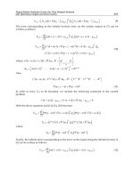
)]()([)dim( susCsiss
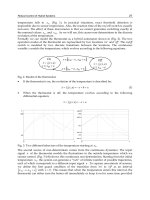
0
(42)
)()()()()( sissLsissLsu
mmmmLm
(43)
)()()()()( ssussCsussCsi
CmmCmmCm
)]([)( ssiR
s
su
mmRm
1
)()()()( susususu
RmCmLm
)()(.)()( siRsi
Cs
su
Ls
si
mmm
mm
m
1111
(45)
Fig. 17. Simulation model for mechanical part
A second model is taken in consideration. The transducer is considered coupled with the
concentrator and the equivalent circuit is presented in Fig. 18.
Fig. 18. Equivalent circuit of the transducer with concentrator
In this model there is a series RLC circuit with the parameters L
m1
, C
m1
and R
m1
for the
transducer T and a series RLC circuit with the parameters L
m2
, C
m2
and R
m2
for the
concentrator C, coupled in cascade. The parts of the control block diagram are modelled
using Simulink blocks. A transient characteristic of the frequency control system is
presented in Fig. 19.
Fig. 19. Transient characteristic for the error, obtained by simulation
The simulation is made considering for the first model the variation with 10 % at the
transducer parameters. The deviation in frequency is eliminated fast. The frequency
response has a small overshoot.
Methodsforparameterestimationandfrequencycontrolofpiezoelectrictransducers 131
signal, generated by a voltage controlled frequency generator GF_CT. The rectangular
command signal u
c
has the frequency f and equal durations of the pulses. The frequency of
the signal u
c
is controlled with the voltage u
f
*. The frequency control system from Fig. 16 is
based on the derivative movement current error e
dim
as the difference between the reference
value dim*=0 and the computed value of the derivative dim:
dimdim
*
dim
e
(40)
A PI controller RG-f is used to control the frequency, with the following transfer function:
)()(
dim
*
se
sT
Ksu
R
Rf
1
1
(41)
The frequency controller is working after the error of the derivative of the movement
current
e
dim
. The derivative of the movement current dim is computed using a circuit
CC_DCM, based on the following relation with Laplace transformations:
where
C
0
is the known constant value of the capacitor from transducer input and u and i are
the measured values of the transducer voltage and current. The voltage upon the transducer
u and the current i through the transducer are measured using a voltage sensor Tu and
respectively a current sensor Ti.
6.3 Modelling and simulation
Two models for the transducer and for the block diagram from Fig. 16 were developed to
test the control principle by simulation. In the first model the parameters of the mechanical
part are considered with a fix static value and a dynamical variation. In the second model
the electromechanical transducer is considered coupled with a mechanical concentrator and
the equivalent circuits are coupled in series. Approximating the relations (41), the following
relations are used to model the behaviour of the piezoelectric transducer:
The mechanic parameters from the above relations have the following variations, in the
vicinity of the stationary points
R
m0
, L
m0
and C
m0
:
mmmmmmmmm
CCCLLLRRR
000
,,
(44)
The movement current
i
m
(s) is modelled, based on the above relations, with the following
relation:
The block diagram of the movement current model is presented in Fig. 17.
)]()([)dim( susCsiss
0
(42)
)()()()()( sissLsissLsu
mmmmLm
(43)
)()()()()( ssussCsussCsi
CmmCmmCm
)]([)( ssiR
s
su
mmRm
1
)()()()( susususu
RmCmLm
)()(.)()( siRsi
Cs
su
Ls
si
mmm
mm
m
1111
(45)
Fig. 17. Simulation model for mechanical part
A second model is taken in consideration. The transducer is considered coupled with the
concentrator and the equivalent circuit is presented in Fig. 18.
Fig. 18. Equivalent circuit of the transducer with concentrator
In this model there is a series RLC circuit with the parameters L
m1
, C
m1
and R
m1
for the
transducer T and a series RLC circuit with the parameters L
m2
, C
m2
and R
m2
for the
concentrator C, coupled in cascade. The parts of the control block diagram are modelled
using Simulink blocks. A transient characteristic of the frequency control system is
presented in Fig. 19.
Fig. 19. Transient characteristic for the error, obtained by simulation
The simulation is made considering for the first model the variation with 10 % at the
transducer parameters. The deviation in frequency is eliminated fast. The frequency
response has a small overshoot.
AUTOMATION&CONTROL-TheoryandPractice132
6.4 Implementation and test results
The frequency control system is developed to be implemented using analogue, high and low
power circuits, for general usage. The power amplifier AP is built using four power IGBT
transistors, in a complete bridge, working in commutation at high frequency. The electric
circuit of the power inverter is presented in Fig. 20.
Fig. 20. The power inverter
The four IGBT transistors V14 have the voltage and current protection circuits. The power
transistors are commanded with 4 circuits Cmd. The Power inverter is fed from the power
system with a rectifier and a filter. The command circuits are receiving the command
voltage u
c
from the VC_FG circuit. The voltage controlled frequency generator GF_CT is
made using a phase lock loop PLL circuit and a comparator. The computing circuit
CC_DCM, which implements the relations and the frequency controller RG-f are realized
using analogue operational amplifiers. The transformer T is realized using ferrite cores,
working at high frequency. The electronic generator is presented in Fig. 21.
Fig. 21. The electronic generator
Some transient signal variations are presented as follows. The pulse train of the command
voltage u
c
is presented in Fig. 22.
Fig. 22. Examples of sensor impulse trains.
The output voltage of the power amplifier is presented in Fig. 23.
Fig. 23. The output voltage
The voltage u over the piezoelectric transducer is presented in Fig. 24.
Fig. 24. The transducer voltage
Methodsforparameterestimationandfrequencycontrolofpiezoelectrictransducers 133
6.4 Implementation and test results
The frequency control system is developed to be implemented using analogue, high and low
power circuits, for general usage. The power amplifier AP is built using four power IGBT
transistors, in a complete bridge, working in commutation at high frequency. The electric
circuit of the power inverter is presented in Fig. 20.
Fig. 20. The power inverter
The four IGBT transistors V14 have the voltage and current protection circuits. The power
transistors are commanded with 4 circuits Cmd. The Power inverter is fed from the power
system with a rectifier and a filter. The command circuits are receiving the command
voltage u
c
from the VC_FG circuit. The voltage controlled frequency generator GF_CT is
made using a phase lock loop PLL circuit and a comparator. The computing circuit
CC_DCM, which implements the relations and the frequency controller RG-f are realized
using analogue operational amplifiers. The transformer T is realized using ferrite cores,
working at high frequency. The electronic generator is presented in Fig. 21.
Fig. 21. The electronic generator
Some transient signal variations are presented as follows. The pulse train of the command
voltage u
c
is presented in Fig. 22.
Fig. 22. Examples of sensor impulse trains.
The output voltage of the power amplifier is presented in Fig. 23.
Fig. 23. The output voltage
The voltage u over the piezoelectric transducer is presented in Fig. 24.
Fig. 24. The transducer voltage
AUTOMATION&CONTROL-TheoryandPractice134
The measured movement current i
m
is presented in Fig. 25.
Fig. 25. The movement current
The control system was developed for a plastic welding machine in the range of 3000 W at
40 kHz.
7. Conclusion
This chapter presented two methods for parameter identification at the piezoelectric
transducers used in high power ultrasonic applications as welding, cleaning and other. The
methods are offering information about the equivalent electrical circuit: parameters and
resonance frequency, efficiency and other. The first parameter estimation method is using
the transformation from non-parameter model – the Nyquist hodograph - to a parameter
model - the transfer function of the transducer’s impedance, testing the piezoelectric
transducers with a sinusoidal signal with variable frequency. The second parameter
estimation method is based on an automatic measurement of piezoelectric transducer
impedance using a deterministic convergence scheme with a gradient method with
continuous adjustment – the method of deepest descent with a maximum slope. Some
practical results are given. Some indications to implement the method using LabView are
given. In the end, the paper provides a method for frequency control at ultrasonic high
power piezoelectric transducers, using a feedback control systems based on the first
derivative of the movement current. This method assures a higher efficiency of the energy
conversion and greater frequency stability. A simulation for two kinds of transducer model
is made. The control principle is implanted on a power electronic generator. Some transient
characteristics are presented. The frequency control system was modelled and simulated
using Matlab and Simulink. Two models for the mechanical part of the transducer are
chosen. Two different regimes for the time variations of the mechanical parameters of the
transducer was chosen and tested. A Simulink model and a simulation result are presented.
The simulation results have proven that the control principle developed in this paper gives
good quality criteria for the output frequency control. The control system is implemented
using a power inverter with transistors working in commutation at high frequencies and
analogue circuits for command. Transient characteristics of the control systems are
presented. The frequency control system may be developed for piezoelectric transducers in
a large scale of constructive types, powers and frequencies, using general usage analogue
components, at a low price, with good control criteria.
8. References
Bose, B.K., (2000). Energy, Environment and Advances in Power Electronics, IEEE
Transactions on Power Electronics, vol. 15, no. 4, July, 2000, pag. 688-701.
Chen, Y. C., Hung, L. C., Chaol, S.H. & Chien, T. H. (2008). PC-base impedance
measurement system for piezoelectric transducers and its implementation on
elements values extraction of lump circuit model, WSEAS Transactions on Systems,
Volume 7, Issue 5, May 2008. Pages 521-526.
Eykhoff, P. (1974). System Identification, John Wiley and Sons, Chicester, U.K., 1974.
Furuichi, S. & Nose, T., (1981). Driving system for an ultrasonic piezoelectric transducer,
U.S. patent 4271371.
Gallego-Juarez, J. A. (2009). Macrosonics: Sound as a Source of Energy, In: Recent Advances
in Accoustic and Music, Theory and Applications, Proceedings of the 10th WSEAS
International Conference on Acoustics & Music Theory & Applications, pag. 11-12, ISBN:
978-960-474-061-1, ISSN 1790-5095, Prague, Czech Rep., March 23-25, 2009.
Hulst, A.P., (1972). Macrosonics in industry 2. Ultrasonic welding of metals, Ultrasonics,
Nov., 1972.
Khmelev, V.N., Barsukov, R.V., Barsukov, V., Slivin, A.N. and Tchyganok, S.N., (2001).
System of phase-locked-loop frequency control of ultrasonic generators, Proceedings
of the 2nd Annual Siberian Russian Student Workshop on
Electron Devices and Materials,
2001. pag. 56-57.
Kirsch, M. & Berens, F., (2006). Automatic frequency control circuit, U. S. Patent 6571088.
Marchesoni, M., (1992). High-Performance Current Control Techniques for Applications to
Multilevel High-Power Voltage Source Inverters, In IEEE Trans. on Power Electronics,
Jan.
Mori, E., 1989. High Power Ultrasonic Wave Transmission System, In J. Inst. Electron. Inf.
Commun. Eng., vol. 72, no. 4, April.
Morris, A.S., (1986). Implementation of Mason's model on circuit analysis programs, In IEEE
Transactions on ultrasonics, ferroelectric and frequency control, vol. UFFC-33, no. 3.
Neppiras, E.A., (1972). Macrosonics in industry, 1. Introduction. Ultrasonics, Jan., 1972.
Prokic, M., (2004). Piezoelectric Converters Modelling and Characterization, MPI Interconsulting,
Le Locle, Switzerland.
Radmanovic, M. D. & Mancic, D. D., (2004). Design and Modelling of Power Ultrasonic
Transducers, University of Nis, 2004, MPI Interconsulting.
Senchenkov, I.K., (1991). Resonance vibrations of an electromechanical rod system with
automatic frequency control, International Applied Mechanics, Vol. 27, No. 9, Sept.,
Springer, N. Y.
Sulivan, R.A. (1983). Power supply having automatic frequency control for ultrasonic
bonding, U. S. Patent 4389601.
Tertisco, M. & Stoica, P. (1980), Identificarea si estimarea parametrilor sistemelor, Editura
Academiei Romaniei, Bucuresti, 1980.
Methodsforparameterestimationandfrequencycontrolofpiezoelectrictransducers 135
The measured movement current i
m
is presented in Fig. 25.
Fig. 25. The movement current
The control system was developed for a plastic welding machine in the range of 3000 W at
40 kHz.
7. Conclusion
This chapter presented two methods for parameter identification at the piezoelectric
transducers used in high power ultrasonic applications as welding, cleaning and other. The
methods are offering information about the equivalent electrical circuit: parameters and
resonance frequency, efficiency and other. The first parameter estimation method is using
the transformation from non-parameter model – the Nyquist hodograph - to a parameter
model - the transfer function of the transducer’s impedance, testing the piezoelectric
transducers with a sinusoidal signal with variable frequency. The second parameter
estimation method is based on an automatic measurement of piezoelectric transducer
impedance using a deterministic convergence scheme with a gradient method with
continuous adjustment – the method of deepest descent with a maximum slope. Some
practical results are given. Some indications to implement the method using LabView are
given. In the end, the paper provides a method for frequency control at ultrasonic high
power piezoelectric transducers, using a feedback control systems based on the first
derivative of the movement current. This method assures a higher efficiency of the energy
conversion and greater frequency stability. A simulation for two kinds of transducer model
is made. The control principle is implanted on a power electronic generator. Some transient
characteristics are presented. The frequency control system was modelled and simulated
using Matlab and Simulink. Two models for the mechanical part of the transducer are
chosen. Two different regimes for the time variations of the mechanical parameters of the
transducer was chosen and tested. A Simulink model and a simulation result are presented.
The simulation results have proven that the control principle developed in this paper gives
good quality criteria for the output frequency control. The control system is implemented
using a power inverter with transistors working in commutation at high frequencies and
analogue circuits for command. Transient characteristics of the control systems are
presented. The frequency control system may be developed for piezoelectric transducers in
a large scale of constructive types, powers and frequencies, using general usage analogue
components, at a low price, with good control criteria.
8. References
Bose, B.K., (2000). Energy, Environment and Advances in Power Electronics, IEEE
Transactions on Power Electronics, vol. 15, no. 4, July, 2000, pag. 688-701.
Chen, Y. C., Hung, L. C., Chaol, S.H. & Chien, T. H. (2008). PC-base impedance
measurement system for piezoelectric transducers and its implementation on
elements values extraction of lump circuit model, WSEAS Transactions on Systems,
Volume 7, Issue 5, May 2008. Pages 521-526.
Eykhoff, P. (1974). System Identification, John Wiley and Sons, Chicester, U.K., 1974.
Furuichi, S. & Nose, T., (1981). Driving system for an ultrasonic piezoelectric transducer,
U.S. patent 4271371.
Gallego-Juarez, J. A. (2009). Macrosonics: Sound as a Source of Energy, In: Recent Advances
in Accoustic and Music, Theory and Applications, Proceedings of the 10th WSEAS
International Conference on Acoustics & Music Theory & Applications, pag. 11-12, ISBN:
978-960-474-061-1, ISSN 1790-5095, Prague, Czech Rep., March 23-25, 2009.
Hulst, A.P., (1972). Macrosonics in industry 2. Ultrasonic welding of metals, Ultrasonics,
Nov., 1972.
Khmelev, V.N., Barsukov, R.V., Barsukov, V., Slivin, A.N. and Tchyganok, S.N., (2001).
System of phase-locked-loop frequency control of ultrasonic generators, Proceedings
of the 2nd Annual Siberian Russian Student Workshop on
Electron Devices and Materials,
2001. pag. 56-57.
Kirsch, M. & Berens, F., (2006). Automatic frequency control circuit, U. S. Patent 6571088.
Marchesoni, M., (1992). High-Performance Current Control Techniques for Applications to
Multilevel High-Power Voltage Source Inverters, In IEEE Trans. on Power Electronics,
Jan.
Mori, E., 1989. High Power Ultrasonic Wave Transmission System, In J. Inst. Electron. Inf.
Commun. Eng., vol. 72, no. 4, April.
Morris, A.S., (1986). Implementation of Mason's model on circuit analysis programs, In IEEE
Transactions on ultrasonics, ferroelectric and frequency control, vol. UFFC-33, no. 3.
Neppiras, E.A., (1972). Macrosonics in industry, 1. Introduction. Ultrasonics, Jan., 1972.
Prokic, M., (2004). Piezoelectric Converters Modelling and Characterization, MPI Interconsulting,
Le Locle, Switzerland.
Radmanovic, M. D. & Mancic, D. D., (2004). Design and Modelling of Power Ultrasonic
Transducers, University of Nis, 2004, MPI Interconsulting.
Senchenkov, I.K., (1991). Resonance vibrations of an electromechanical rod system with
automatic frequency control, International Applied Mechanics, Vol. 27, No. 9, Sept.,
Springer, N. Y.
Sulivan, R.A. (1983). Power supply having automatic frequency control for ultrasonic
bonding, U. S. Patent 4389601.
Tertisco, M. & Stoica, P. (1980), Identificarea si estimarea parametrilor sistemelor, Editura
Academiei Romaniei, Bucuresti, 1980.
AUTOMATION&CONTROL-TheoryandPractice136
Volosencu, C. (2008). Frequency Control of the Pieozoelectric Transducers, Based on the
Movement Current, Proceedings of ICINCO 2008 – Fifth International Conference on
Informatics in Control, Automation and Robotics, ISBN 978-989-8111-35-7, Funchal,
Madeira, Portugal, May 11-15, 2008.
DesignoftheWaveDigitalFilters 137
DesignoftheWaveDigitalFilters
BohumilPsenicka,FranciscoGarcíaUgaldeandAndrésRomeroM.
X
Design of the Wave Digital Filters
Bohumil Psenicka, Francisco García Ugalde and Andrés Romero M.
Universidad Nacional Autónoma de México
México
1. Introduction
In control automation and robotics filters are used in image processing, in the automatics of
alarm system, adaptive signal processing and control vibration, as well as in the control of
mobile robots, system identification, speech system recognition, etc.
In this chapter “Design of the Wave Digital filters” we shall propose a very simple
procedure for designing, analysis and realization of low-pass, high-pass, band-pass and
band-stop wave digital filters from reference LC filters given in the lattice configuration and
will be introduced tables for simple design of the wave digital filters.
Wave digital filters are derived from LC-filters. The reference filter consists of parallel and
serial connections of several elements. Since the load resistance R is not arbitrary but
dependent on the element or source to which the port belongs, we cannot simply
interconnect the elements to a network. The elements of the filters are connected with the
assistance of serial and parallel adaptors. This adaptors in the discrete form are connected in
one port by delay elements. The possibility of changing the port resistance can be achieved
using parallel and serial adaptors. These adaptors contain the necessary adders, multipliers
and inverters.
2. Serial and parallel adaptors.
In this chapter, we use adaptors with three ports. Blocks the serial and parallel reflection-
free adapters and theirs signal-flow diagram are shown in figure 1.
The coefficient of the 3-port reflection-free serial adaptor in figure 1A) is calculated from the
port resistances R
i
i=1,2 by (1).
(1)
The coefficient of the reflection-free parallel adaptor in figure 1B) can be calculated from the
port conductance G
i
i=1,2 by (2)
(2)
9
AUTOMATION&CONTROL-TheoryandPractice138
Fi
g
B)
T
h
co
n
T
h
p
o
Fi
g
pa
W
h
de
ca
n
g
. 1. A) Three po
r
Three port paral
l
h
e coefficients of
n
ductances G
i
i
=
h
e coefficients of
o
rt resistances R
i
g
. 2. A) Three-p
rallel depende
n
t
h
en connectin
g
a
la
y
element in
o
n
not connect the
r
t serial adaptor
w
l
el adaptor whos
e
the dependent
p
=
1,2,3 by (3)
A
G
1
1
2
the dependent s
e
i=1,2,3 by (4)
B
R
1
1
2
p
ort serial depe
n
adaptor and its
s
a
daptors, the ne
t
o
rder to
g
uarant
e
dependent ada
p
w
hose port 3 is
r
e
port 3 is reflect
i
p
arallel adaptor
G
A
G G
G
1
2
2 3
2
e
rial adaptor in
t
R
B
R R R
1
2
2 3 1
2
n
dent adaptor a
n
s
i
g
nal flow
g
rap
h
t
work must not
e
e that the stru
c
p
tors from figur
e
r
eflectio
n
-free an
d
i
o
n
-free and its s
i
in the fi
g
ure 2B
)
G
G
G G
2
1 2 3
2
t
he fi
g
ure 2A) ca
n
R
R R
2
2 3
2
n
d its signal-flo
w
h
.
contain an
y
fee
d
c
ture is realizabl
e
e
2A) and 2B). T
h
d
its si
g
nal flow-
ig
nal flow-
g
raph
.
)
can be
g
et fro
m
n
be obtained fr
o
w
graph, B)Thr
e
d
back loops wit
h
e
. This means t
h
h
e free-port dep
e
graph,
.
m
port
(3)
o
m the
(4)
e
e-port
h
out a
h
at we
e
ndent
pa
re
f
3.
B
y
di
g
ac
c
w
a
sa
m
4.
In
In
an
Fi
g
co
n
Fi
r
co
e
de
rallel is reflecti
o
f
lection free if R
3
=
Examples
y
means of exam
p
g
ital filters. The
c
ordin
g
to Fett
w
a
ve di
g
ital struc
t
m
plin
g
frequenc
y
Realization of
the first exampl
e
the fi
g
ure 3 we
d its correspond
i
g
. 3.
LC refere
n
n
nection.
r
st we must cal
c
e
fficients of the
p
pendent parallel
o
n free at port 3 i
f
=
R
1
+R
2
.
p
les we shall de
m
most important
w
eis procedure (
F
t
ures was desi
gn
y
f
s
=0.5
the low-pas fi
e
we shall realiz
e
show the struct
u
i
n
g
block connec
t
n
ce Butterworth
c
ulate from
f
i
g
u
r
p
arallel and seri
a
adaptor A
51
,A
52
a
f
G
3
= G
1
+G
2
an
d
m
onstrate calcula
t
components fo
r
F
ettweis 1972) a
r
n
ed for the cor
n
lter.
e
a Butterworth l
o
u
re of a 5
th
order
t
ion in the di
g
ital
low-pass filter
r
e 3 (G
0
=1) wa
v
a
l adaptors A
1
,B
2
,
a
ccordin
g
to (1)-
(
d
three-port dep
e
t
ion of the low-p
a
r
the realization
r
e the ladder L
C
n
er frequenc
y
f
1
o
w-pass of the 5
t
h
ladder LC refer
e
form.
and its corres
p
v
e port resistanc
e
,
A
3
,B
4
and finall
y
(
3).
e
ndent serial ad
a
a
ss and high-pas
s
of wave di
g
ital
C
filters. The tab
=1/(2pi)=0.1591
5
h
order and A
ma
x
e
nce Butterwort
h
p
ondin
g
di
g
ital
e
s R
1
,R
2
,R
3
,R
4
th
y
the coefficients
a
ptor is
s
wave
filters
les for
5
5 and
x
=3 dB.
h
filter
block
e
n
the
of the
DesignoftheWaveDigitalFilters 139
Fi
g
B)
T
h
co
n
T
h
p
o
Fi
g
pa
W
h
de
ca
n
g
. 1. A) Three po
r
Three port paral
l
h
e coefficients of
n
ductances G
i
i
=
h
e coefficients of
o
rt resistances R
i
g
. 2. A) Three-
p
rallel depende
n
t
h
en connectin
g
a
la
y
element in
o
n
not connect the
r
t serial adaptor
w
l
el adaptor whos
e
the dependent
p
=
1,2,3 b
y
(3)
A
G
1
1
2
the dependent s
e
i=1,2,3 by (4)
B
R
1
1
2
p
ort serial depe
n
adaptor and its
s
a
daptors, the ne
t
o
rder to
g
uarant
e
dependent ada
p
w
hose port 3 is
r
e
port 3 is reflect
i
p
arallel adaptor
G
A
G G
G
1
2
2 3
2
e
rial adaptor in
t
R
B
R R R
1
2
2 3 1
2
n
dent adaptor a
n
s
i
g
nal flow
g
rap
h
t
work must not
e
e that the stru
c
p
tors from fi
g
ur
e
r
eflectio
n
-free an
d
i
o
n
-free and its s
i
in the fi
g
ure 2B
)
G
G
G G
2
1 2 3
2
t
he fi
g
ure 2A) ca
n
R
R R
2
2 3
2
n
d its si
g
nal-flo
w
h
.
contain an
y
fee
d
c
ture is realizabl
e
e
2A) and 2B). T
h
d
its si
g
nal flow-
ig
nal flow-
g
raph
.
)
can be
g
et fro
m
n
be obtained fr
o
w
g
raph, B)Thr
e
d
back loops wit
h
e
. This means t
h
h
e free-port dep
e
graph,
.
m
port
(3)
o
m the
(4)
e
e-port
h
out a
h
at we
e
ndent
pa
re
f
3.
B
y
di
g
ac
c
w
a
sa
m
4.
In
In
an
Fi
g
co
n
Fi
r
co
e
de
rallel is reflecti
o
f
lection free if R
3
=
Examples
y
means of exam
p
g
ital filters. The
c
ordin
g
to Fett
w
a
ve di
g
ital struc
t
m
plin
g
frequenc
y
Realization of
the first exampl
e
the fi
g
ure 3 we
d its correspond
i
g
. 3.
LC refere
n
n
nection.
r
st we must cal
c
e
fficients of the
p
pendent parallel
o
n free at port 3 i
f
=
R
1
+R
2
.
p
les we shall de
m
most important
w
eis procedure (
F
t
ures was desi
gn
y
f
s
=0.5
the low-pas fi
e
we shall realiz
e
show the struct
u
i
n
g
block connec
t
n
ce Butterworth
c
ulate from
f
i
g
u
r
p
arallel and seri
a
adaptor A
51
,A
52
a
f
G
3
= G
1
+G
2
an
d
m
onstrate calcula
t
components fo
r
F
ettweis 1972) a
r
n
ed for the cor
n
lter.
e
a Butterworth l
o
u
re of a 5
th
order
t
ion in the di
g
ital
low-pass filter
r
e 3 (G
0
=1) wa
v
a
l adaptors A
1
,B
2
,
a
ccordin
g
to (1)-
(
d
three-port dep
e
t
ion of the low-p
a
r
the realization
r
e the ladder L
C
n
er frequenc
y
f
1
o
w-pass of the 5
t
h
ladder LC refer
e
form.
and its corres
p
v
e port resistanc
e
,
A
3
,B
4
and finall
y
(
3).
e
ndent serial ad
a
a
ss and high-pas
s
of wave di
g
ital
C
filters. The tab
=1/(2pi)=0.1591
5
h
order and A
ma
x
e
nce Butterwort
h
p
ondin
g
di
g
ital
e
s R
1
,R
2
,R
3
,R
4
th
y
the coefficients
a
ptor is
s
wave
filters
les for
5
5 and
x
=3 dB.
h
filter
block
e
n
the
of the
AUTOMATION&CONTROL-TheoryandPractice140
T
h
fo
l
pr
o
st
r
Fi
g
A
1
N
G
R
1
1
h
e pro
g
ram for t
h
l
lows, and the f
r
og
ram for com
p
r
ucture in the fi
gu
g
. 4. Butterworth
1
=0.618146;B2=0.
2
N
2=0; N4=0; N6=
0
G C .
.
G
R R L
G
R
G
A
G C
G
A
G C
G
A
G C
G
0 1
1
2 1 2
2
2
0
1
0 1
2
3
2 3
4
51
4 5
1 618
1
0 618
1
2
h
e anal
y
sis o
f
th
e
r
equenc
y
respo
n
p
utin
g
XN1-XN
4
u
re 4.
wave di
g
ital lo
w
2
76524;A3=0.182
8
0
; N8=0; N10=0;
X
.
.
.
.
.
A
G
5
2 236
0 447
0 618
0 182
0 467
e
wave di
g
ital fil
t
n
se obtained is
g
4
, BN4-BN1,N1-
N
w
-pass filter of th
e
8
58;B4=0.201756;
A
X
N=1
G G C
R .
G
R R L
G .
R
R
B
R L
R
B
R L
G
A
G C
3 2 3
3
3
4 3 4
4
4
1
2
1 2
3
4
3 4
5
52
4
2
1
0
4
2
1
0
4
0
0
2
G
5 5
t
er of the 5
th
ord
g
iven in fi
g
ure
4
N
9 and YN(i)
w
e
5
th
order.
A
51=0.467353;A
5
.
.
.
.
2
447
4
08
026
4
93
276
0
201
.0 947
er written in M
A
4
. The equation
w
as obtained fr
o
5
2=0.947276;
A
TLAB
in the
o
m the
Fi
g
5.
A
s
fil
t
A
3
ch
a
hi
g
pr
o
for i=1:1:200
XN1=A1*X
N
XN3=N6-
A
BN4=XN
4
BN3=XN
3
BN2=XN
2
BN1=XN1
N1=XN*
A
N5=BN3-
A
N9=N10-
A
YN(i)=2*
N
N2=N1;N4
=
end
[h,w]=freqz(Y
N
Plot(w,20*lo
g
10
g
. 5. Frequenc
y
r
e
Design of the
s
a second exam
p
t
er for n=5, A
max
=0.182, B
4
=0.19
2
a
n
g
in
g
the valu
e
g
h-pass filter in
og
ram we also h
a
N
-A1*N2+N2;
A
3*XN2-A3*N6;
4
-A51*XN4+2*N1
3
-B4*XN4-B4*BN
4
2
-A3*XN2+BN3+
N
-BN2*XN2-B2*B
N
A
1-A1*N2+BN1;
A
3*XN2-A3*N6;
A
51*XN4-A51*N
1
N
10-A51*XN4-A5
=
N3;N6=N5;N8=
N
N
,1,200)
(abs(h)))
e
sponse in dB of
t
low-pass and
p
le we shall pr
o
=3 dB. From tab
2
, A
51
=0.383 an
d
e
s of the coeffici
e
the fi
g
ure 6. A
d
a
ve to chan
g
e N
2
XN2=XN1+N
4
XN4=XN3+
N
0-A51*N10-A52*
N
4
;
N
6-A3*N6;
N
2;
N3=BN1+BN
2
N7=BN3+BN
4
1
0-A52*N10;
1*N10-A52*N10;
N
7;N10=N9;XN
=
t
he Butterworth
l
high-pass Ch
e
o
pose low-pass a
n
le 7 we
g
et the
v
d
A
52
=0.360. Us
i
e
nts we
g
et the a
t
d
ditionall
y
to
g
et
2
= -N1; N4= -N3;
4
;
N
8;
N
10;
2
;
4
;
=
0;
l
ow-pass filter
.
e
bychev filter
n
d high-pass C
h
v
alues of the W
D
i
n
g
previous
M
t
tenuation of C
h
the hi
g
h-pass f
i
N6= -N5; N8= -
N
h
eb
y
chev wave
D
F A
1
=0.223, B
2
=
M
ATLAB pro
g
ra
m
h
eb
y
chev low-pa
i
lter from the pr
N
7; N10= -N9.
digital
=
0.226,
m
and
ss and
evious