Channel Characteristics
Bạn đang xem bản rút gọn của tài liệu. Xem và tải ngay bản đầy đủ của tài liệu tại đây (341.44 KB, 31 trang )
4
Channel Characteristics
4.1 Introduction
This chapter considers the propagation environment in which a mobile-satellite system oper-
ates. The space between the transmitter and receiver is termed the channel. In a mobile-
satellite network, there are two types of channel to be considered: the mobile channel,
between the mobile terminal and the satellite; and the fixed channel, between the fixed
Earth station or gateway and the satellite. These two channels have very different character-
istics, which need to be taken into account during the system design phase. The more critical
of the two links is the mobile channel, since transmitter power, receiver gain and satellite
visibility are restricted in comparison to the fixed-link. The basic transmission chain is shown
in Figure 4.1.
By definition, the mobile terminal operates in a dynamic, often hostile environment in
which propagation conditions are constantly changing. In a mobile’s case, the local opera-
tional environment has a significant impact on the achievable quality of service (QoS). The
different categories of mobile terminal, be it land, aeronautical or maritime, also each have
their own distinctive channel characteristics that need to be considered. On the contrary, the
fixed Earth station or gateway can be optimally located to guarantee visibility to the satellite
at all times, reducing the effect of the local environment to a minimum. In this case, for
frequencies above 10 GHz, natural phenomena, in particular rain, govern propagation impair-
ments. Here, it is the local climatic variations that need to be taken into account. These very
different environments translate into how the respective target link availabilities are specified
for each channel. In the mobile-link, a service availability of 80–99% is usually targeted,
whereas for the fixed-link, availabilities of 99.9–99.99% for the worst-month case can be
specified.
The following reviews the current status of channel modelling from a mobile and a fixed
perspective.
4.2 Land Mobile Channel Characteristics
4.2.1 Local Environment
Spurred on by the needs of the mobile-satellite industry, the 10 years spanning the mid-1980s
Mobile Satellite Communication Networks. Ray E. Sheriff and Y. Fun Hu
Copyright q 2001 John Wiley & Sons Ltd
ISBNs: 0-471-72047-X (Hardback); 0-470-845562 (Electronic)
to the mid-1990s witnessed significant effort around the world in characterising the land
mobile-satellite channel. The vast majority of these measurement campaigns were focused
on the UHF and L-/S-bands, however, by the mid-1990s, with a number of mobile-satellite
systems in operation, focus had switched to characterising the next phase in mobile-satellite
development, that of broadband technology at the Ka-band and above.
The received land mobile-satellite signal consists of the combination of three components:
the direct line-of-sight (LOS) wave, the diffuse wave and the specular ground reflection. The
direct LOS wave arrives at the receiver without reflection from the surrounding environment.
The only L-/S-band propagation impairments that significantly affect the direct component
are free space loss (FSL) and shadowing. FSL is related to operating frequency and transmis-
sion distance. This will be discussed further in the following chapter. Tropospheric effects
can be considered negligible at frequencies below 10 GHz, while impairments introduced by
the ionosphere, in particular, Faraday rotation can be effectively counteracted by the selec-
tive use of transmission polarisation. Systems operating at above 10 GHz need to take into
account tropospheric impairments and these will be considered further when discussing the
fixed-link channel characteristics.
Shadowing occurs when an obstacle, such as a tree or a building, impedes visibility to the
satellite. This results in the attenuation of the received signal to such an extent that transmis-
sions meeting a certain QoS may not be possible.
The diffuse component comprises multipath reflected signals from the surrounding envir-
onment, such as buildings, trees and telegraph poles. Unlike terrestrial mobile networks,
Mobile Satellite Communication Networks116
Figure 4.1 Mobile network propagation environment.
which rely on multipath propagation, multipath has only a minor effect on mobile-satellite
links in most practical operating environments [VUC-92].
The specular ground component is a result of the reception of the reflected signal from the
ground near to the mobile. Antennas of low gain, wide beamwidth operating via satellites
with low elevation angle are particularly susceptible to this form of impairment. Such a
scenario could include hand-held cellular like terminals operating via a non-geostationary
satellite, for example.
The first step towards modelling the mobile-satellite channel is to identify and categorise
typical transmission environments [VUC-92]. This is usually achieved by dividing the envir-
onment into three broad categories:
†
Urban areas, characterised by almost complete obstruction of the direct wave.
†
Open and rural areas, with no obstruction of the direct wave.
†
Suburban and tree shadowed environments, where intermittent partial obstruction of the
direct wave occurs.
As far as land mobile-satellite systems are concerned, it is the last two of the above
environments that are of particular interest. In urban areas, visibility to the satellite is difficult
to guarantee, resulting in the multipath component dominating reception. Thus, at the mobile,
a signal of random amplitude and phase is received. This would be the case unless multi-
satellite constellations are used with a high guaranteed minimum elevation angle. Here,
satellite diversity techniques allowing optimum reception of one or more satellite signals
could be used to counteract the effect of shadowing.
The fade margin specifies the additional transmit power that is needed in order to compen-
sate for the effects of fading, such that the receiver is able to operate above the threshold or the
minimum signal level that is required to satisfy the performance criteria of the link. The
threshold value is determined from the link budget, which is discussed in the following
chapter. The urban propagation environment places severe constraints on the mobile-satellite
network. For example, in order to achieve a fade margin in the region of 6–10 dB in urban and
rural environments, a continuous guaranteed minimum user-to-satellite elevation angle of at
least 508 is required [JAH-00]. The compensation for such a fade margin should not be
beyond the technical capabilities of a system and could be incorporated into the link design.
However, to achieve such a high minimum elevation angle using a low Earth orbit constella-
tion would require a constellation of upwards of 100 satellites. On the other hand, for a
guaranteed minimum elevation angle of 208, a fade margin in the region of 25–35 dB,
would be required for the same grade of service, which is clearly unpractical. While these
figures demonstrate the impracticalities of providing coverage in urban areas, in reality, for an
integrated space/terrestrial environment, in an urban environment, terrestrial cellular cover-
age would take priority and this is indeed how systems like GLOBALSTAR operate.
In open and rural areas, where direct LOS to the satellite can be achieved with a fairly high
degree of certainty, the multipath phenomenon is the most dominant link impairment. The
multipath component can either add constructively (resulting in signal enhancement) or
destructively (causing a fade) to the direct wave component. This results in the received
mobile-satellite transmissions being subject to significant fluctuations in signal power.
In tree shadowed environments, in addition to the multipath effect, the presence of trees
will result in the random attenuation of the strength of the direct path signal. The depth of the
fade is dependent on a number of parameters including tree type, height, as well as season due
Channel Characteristics 117
to the leaf density on the trees. Whether a mobile is transmitting on the left or right hand side
of the road could also have a bearing on the depth of the fade [GOL-89, PIN-95], due to the
LOS path length variation through the tree canopy being different for each side of the road.
Fades of up to 20 dB at the L-band have been reported due to shadowing caused by roadside
trees in a suburban environment [GOL-92].
In suburban areas, the major contribution to signal degradation is caused by buildings and
other man-made obstacles. These obstacles manifest as shadowing of the direct LOS signal,
resulting in attenuation of the received signal. The motion of the mobile through suburban
areas results in the continuous variation in the received signal strength and variation in the
received phase.
The effect of moving up in frequency to the K-/Ka-bands imposes further constraints on the
design of the link. Experimental measurement campaigns performed in Southern California
by the jet propulsion laboratory as part of the Advanced Communications Technologies
Satellite (ACTS) (not to be confused with the European ACTS R&D Programme) Mobile
Programme reported results for three typical transmission environments [PIN-95]. For an
environment in which infrequent, partial blocking of the LOS component occurred, fade
depths of 8, 1 and 1 dB were measured at the K-band, corresponding to fade levels of 1, 3
and 5%, respectively. This implies that for 1% of the time, the faded received signal is greater
than 8 dB below the reference pilot level and so on. In an environment in which occasional
complete shadowing of the LOS component occurred, corresponding fade depths of 27, 17.5
and 12.5 dB were measured. Lastly, for an environment in which frequent complete blockage
of the LOS occurred, fade depths of greater than 30 dB were obtained for as low as a 5% fade
level. In all environments, fade depths at the K- and Ka-bands were found to be essentially the
same. Similar degrees of fading were found during European measurement campaigns, such
as under the European Union’s ACTS programme SECOMS project. The results demonstrate
the difficulty in providing reliable mobile communications to any environment in which the
LOS to the satellite may be restricted.
Channel modelling is classified into two categories: narrowband and wideband. In the
narrowband scenario, the influence of the propagation environment can be considered to
be the same or similar for all frequencies within the band of interest. Consequently, the
influence of the propagation medium can be characterised by a single, carrier frequency.
In the wideband scenario, on the other hand, the influence of the propagation medium does
not affect all components occupying the band in a similar way, thus causing distortion to
selective spectral components.
4.2.2 Narrowband Channel Models
4.2.2.1 Overview
Narrowband channel characterisation is primarily aimed at establishing the amplitude
variation of the signal transmitted through the channel. The vast majority of measurement
campaigns have used the narrowband approach and, consequently, a number of narrowband
models have been proposed. These models can be classified as being either (a) empirical with
regression line fits to measured data, (b) statistical or (c) geometric-analytical.
Empirical models can be used to characterise the sensitivity of the results to critical
parameters, e.g. elevation angle, frequency. Statistical models such as the Rayleigh, Rician
and log-normal distributions or their combinations for use in different transmission environ-
Mobile Satellite Communication Networks118
ments, are especially useful for software simulation analysis; whilst geometric-analytical
models provide an understanding of the transmission environment, through the modelling
of the topography of the environment.
4.2.2.2 Empirical Regression Models
A number of measurement campaigns performed throughout the world have aimed to cate-
gorise the mobile-satellite channel. These measurement campaigns have attempted to
emulate the satellite by using experimental air borne platforms, that is helicopters, aircraft,
air balloons, or in some cases existing geostationary satellite systems have been used. The
following briefly describes some of the most widely cited models.
Empirical Roadside Shadowing (ERS) Model This model is used to characterise the
effect of fading predominantly due to roadside trees. The model is based upon
measurements performed in rural and suburban environments in central Maryland, US,
using helicopter-mobile and satellite-mobile links at the L-band [VOG-92]. Measurements
were performed for elevation angles in the range 20–608; the 208 measurements utilised a
mobile-satellite link, and the remainder a helicopter. The subsequent empirical expression
derived from the measurement campaign for a frequency of 1.5 GHz is given by
A
L
ðP;
u
; f
L
Þ¼2Mð
u
ÞlnP 1 Nð
u
Þ dB for f
L
¼ 1:5GHz ð4:1Þ
Mð
u
Þ¼a 1 b
u
1 c
u
2
ð4:2Þ
Nð
u
Þ¼d
u
1 e ð4:3Þ
a ¼ 3:44; b ¼ 0:0975; c ¼ 20:002; d ¼ 20:443 and e ¼ 34:76 ð4:4Þ
where A
L
(P,
u
,f
L
) denotes the value of the fade exceeded in decibels, L denotes the L-band, f
L
is the frequency at L-band in GHz and is equal to 1.5 GHz in the equation; P is the percentage
of the distance travelled over which the fade is exceeded (in the range 1–20%) or the outage
Channel Characteristics 119
Table 4.1 ERS model characteristics
Elevation
angle (8)
M(
u
) N(
u
)
20 4.59 25.90
25 4.63 23.69
30 4.57 21.47
35 4.40 19.26
40 4.14 17.04
45 3.78 14.83
50 3.32 12.61
55 2.75 10.40
60 2.09 8.18
probability in the range of 1–20% for a given fade margin.
u
is the elevation angle. From
the above, the following model characteristics can be derived (Table 4.1).
The following relationship between UHF and L-band has been derived for fade depth in
tree shadowed areas for P in the range of 1–30% [VOG-88].
A
L
ðP;
u
; f
L
Þ¼A
uhf
ðP;
u
; f
uhf
Þ
ffiffiffiffiffiffi
f
L
f
uhf
s
dB ð4:5Þ
Similarly, it was found that when scaling from L-band (1.3 GHz) to S-band (2.6 GHz) the
following relationship applies:
A
s
ðP;
u
; f
s
Þ < 1:41A
L
ðP;
u
; f
L
Þ dB ð4:6Þ
The ERS model can be found in Ref. [ITU-99a], which provides formulae that can be used
to extend the operational range of the model. The conversion from L-band to K-band and vice
versa in the frequency range 850 MHz to 20 GHz can be obtained from the formula, for an
outage probability within the range 20% $ P $ 1% [ITU-99a]:
A
K
ðP;
u
; f
K
Þ¼A
L
ðP;
u
; f
L
Þexp 1:5
1
ffiffiffi
f
L
p
2
1
ffiffiffi
f
K
p
dB ð4:7Þ
Mobile Satellite Communication Networks120
Figure 4.2 Fading at 1.5 GHz due to roadside shadowing versus path elevation angle.
Elevation angles below 208 down to 78 are assumed to have the same value of fade as that at
208. Figure 4.2 shows the results of application of the ERS model at 1.5 GHz for a range of
elevation angles.
To increase the percentage of distance travelled (or outage probability) to the limits of
80% $ P $ 20%, the ITU recommends the following formula:
A
L2K
ðP;
u
; f
L2K
Þ¼A
K
ð20%;
u
; f
K
Þ
1
ln4
ln
80
P
ð4:8Þ
where A
L2K
() denotes the attenuation for frequencies between 0.85 and 20 GHz.
An extension to the ERS model is also provided for elevation angles greater than 608 at
frequencies of 1.6 and 2.6 GHz, respectively [ITU-99a]. This is achieved by applying the
ERS model for an elevation angle of 608 and then linearly interpolating between the calcu-
lated 608 value and the fade values for an 808 elevation angle given in Table 4.2. Linear
interpolation should also be performed between the figures given in Table 4.2 and 908
elevation, for which the fade exceeded is assumed to be 0 dB.
As noted earlier, the season of operation effects the degree of attenuation experienced by
the transmission. The following expression is used to take into account the effect of foliage on
trees, at UHF, for P in the range 1–30%, indicating a 24% increase in attenuation due to the
presence of leaves.
Aðfull foliageÞ¼1:24Aðno foliageÞ dB ð4:9Þ
The Modified Empirical Roadside Shadowing (MERS) Model The European Space
Agency modified the ERS model in order to increase the elevation angle range up to 808
and the percentage of optical shadowing up to 80%. One form of the MERS is given by
AðP;
u
ÞlnðPÞ 1 Bð
u
Þ dB ð4:10Þ
where P and
u
are as in the ERS model. A(
u
) and B(
u
) are defined by:
Að
u
Þ¼a
1
u
2
1 a
2
u
1 a
3
Channel Characteristics 121
Table 4.2 Fades exceed (dB) at
808 elevation [ITU-99a]
P (%) Tree-shadowed
1.6 GHz 2.6 GHz
1 4.1 9.0
5 2.0 5.2
10 1.5 3.8
15 1.4 3.2
20 1.3 2.8
30 1.2 2.5
a
1
¼ 1:117 £ 10
24
; a
2
¼ 20:0701; a
3
¼ 6:1304
Bð
u
Þ¼b
1
u
2
1 b
2
u
1 b
3
b
1
¼ 0:0032; b
2
¼ 20:6612; b
3
¼ 37:8581
Empirical Fading Model This model is based upon the measurements performed by the
University of Surrey, UK, simultaneously using three bands (L, S and Ku) [BUT-92].
Elevation angles were within the range 60–808. Its basic form is similar to the ERS model
with the addition of a frequency-scaling factor. It is given by
MðP;
u
; fÞ¼að
u
; fÞlnðPÞ 1 cð
u
; fÞð4:11Þ
where
að
u
; fÞ¼0:029
u
2 0:182f 2 6:315
cð
u
; fÞ¼20:129
u
1 1:483f 1 21:374
The model is valid for the following ranges: P, link outage probability, 1–20%; f,
frequency, 1.5–10.5 GHz;
u
, elevation angle, 60–808.
The model has been extended by combining it with the ERS, resulting in the combined
EFM (CEFM) model. This is valid for elevation angles in the range 20–808 with regression
coefficients:
að
u
; fÞ¼0:002
u
2
2 0:15
u
2 0:2f 2 0:7
cð
u
; fÞ¼20:33
u
1 1:5f 1 27:2
4.2.2.3 Probability Distribution Models
Probability distribution models can be used to describe and characterise, with some degree of
accuracy, the multipath and shadowing phenomena. This form of modelling allows the
dynamic nature of the channel to be modelled. In turn, this enables the performance of the
system to be evaluated for different environments. Essentially, a combination of three prob-
ability density functions (PDF) are used to characterise the channel: Rician (when a direct
wave is present and is dominant over multipath reception), Rayleigh (when no direct wave is
present and multipath reception is dominant) and log-normal (for shadowing of the direct
wave when no significant multipath reception is present).
Complete Obstruction of the Direct Wave In an urban environment, the received signal is
characterised by virtually a complete obstruction of the direct wave. In this case, the received
signal will be dominated by multipath reception. The received signal comprises, therefore, of
the summation of all diffuse components. This can be represented by two orthogonal
independent voltage phasors, X and Y, which arrive with random phase and amplitude. The
phase of the diffuse component can be characterised by a uniform probability density function
within the range 0–2
p
, while the amplitude can be categorised by a Rayleigh distribution of
the form
Mobile Satellite Communication Networks122
P
Rayleigh
ðrÞ¼
r
s
2
m
exp 2
r
2
2
s
2
m
!
ð4:12Þ
where r is the signal envelope given by:
r ¼
ffiffiffiffiffiffiffiffiffi
x
2
1 y
2
q
ð4:13Þ
and
s
2
m
is the mean received scattered power of the diffuse component due to multipath
propagation.
As noted in Chapter 1, for an unmodulated carrier, f
c
, the Do
¨
ppler shift, f
d
, of a diffuse
component arriving at an incident angle
u
i
is given by:
f
d
¼
vf
c
c
cos
u
i
Hz ð4:14Þ
where
u
i
is in the range 0–2
p
. This results in a maximum Do
¨
ppler shift f
m
of ^ vf
c
/c, where c
is the speed of light (<3 £ 10
8
m/s).
Hence, at the receiver, a band of signals is received within the range f
c
^ f
m
, where f
m
is
termed the fade rate. For uniform received power for all angles of arrival at the terminal, the
resultant power spectral density is given by the expression:
SðfÞ¼
s
2
m
p
f
m
1 2
ðf 2 f
c
Þ
f
m
2
"#
2
1
2
ðW=HzÞð4:15Þ
Unobstructed Direct Wave When in the presence of a direct source or wave of amplitude
A, as in the mobile-satellite case in an open environment, the representation of the two-
dimensional probability density function of the received voltage is given by [GOL-92]:
P
XY
ðx; yÞ¼
1
2
ps
2
m
exp 2
ðx 2 AÞ
2
1 y
2
2
s
2
m
!
ð4:16Þ
Using the above expression, the p.d.f. of the random signal envelope follows a Rician
distribution:
P
Rice
ðrÞ¼
r
s
2
m
exp 2
r
2
1 A
2
2
s
2
m
!
I
0
rA
s
2
m
ð4:17Þ
where I
0
(.) is the modified zero-order Bessel function of the first kind; A
2
/2 is the mean
received power of the direct wave component, r is the signal envelope and
s
2
m
is the mean
received scattered power of the diffuse component due to multipath propagation.
It can be seen from the above equation that the Rayleigh distribution is a special case of the
Rician distribution and arises when no LOS component is available, i.e. A ¼ 0.
The power ratio of the direct wave to that of the diffuse component, A
2
/2
s
2
m
, is known as
the Rice-factor, which is usually expressed in dB.
Typical values of the Rice-factor, based on measurements in the US and Australia, are
within the range 10–20 dB, with a fade rate of less than 200 Hz for a mobile travelling at less
than 100 km/h [VUC-92]. Rician models can be used when an unobstructed LOS component
Channel Characteristics 123
is present along with coherent and incoherent multipath signals, such as occurs in open rural
areas, for example.
Partial-Shadowing of the Direct Wave The log-normal density function is used to
characterise the effect of shadowing of the direct wave, where no multipath component is
present, here
P
Log-normal
ðrÞ¼
1
s
s
r
ffiffiffiffi
2
p
p
exp 2
ðlnr 2
m
s
Þ
2
2
s
2
s
!
ð4:18Þ
where
s
s
is the standard deviation of the shadowed component (ln r) and m
s
is the mean of the
shadowed component (ln r).
The suburban environment is one in which random shadowing of the direct-wave occurs,
due to the presence of trees, buildings, and so on. The log-normal distribution is used to
model the effect of this environment on the direct wave component, however, a Rayleigh
distribution needs also to be considered in order to take into account the multipath, diffuse
component.
There is no set rule as to what parameters should be applied to the above models in order to
generate a suitable representation of the environment of concern. How the above statistical
models are combined to characterise the complete transmission environment is what identi-
fies a particular model.
Two of the most widely referenced statistical models are those developed by Loo [LOO-
85] and Lutz [LUT-91]. The modellers, however, differ in their approach. The Loo model is
an example of how the constituents of the channel are combined into a single probability
distribution with associated parameters. The Lutz approach, on the other hand, employs state-
orientated statistical modelling, whereby each particular state of the channel is separately
characterised by a probability distribution, with a specified probability of occurrence.
Joint Probability Distribution Modelling Loo’s model is based upon a measurement
campaign performed in Canada using a helicopter to mobile transmission link in rural
environments. The model is valid for elevation angles up to 308. Loo assumed: (a)
received voltage due to diffusely scattered components is Rayleigh distributed; (b) voltage
variations due to attenuation of the direct path signal are log-normally distributed. Further
details can be found in Ref. [LOO-85].
Loo’s PDF for a signal envelope r is given by:
p
Loo
ðrÞ¼
r
s
2
m
ffiffiffiffiffiffiffi
2
ps
2
s
p
Z
1
0
1
A
exp 2
ðlnA 2
m
s
Þ
2
2
s
2
s
2
r
2
1 A
2
2
s
2
m
0
@
1
A
I
0
rA
s
2
m
dA ð4:19Þ
where
s
2
m
is the mean received scattered power of the diffuse component due to multipath
propagation,
s
s
is the standard deviation of the shadowed component (ln A) and m
s
is the
mean of the shadowed component (ln A).
The above expression can be simplified to either (4.18) when r is much greater than
s
m
or
(4.12) when r is much less than
s
m
. Otherwise the above expression needs to be determined
mathematically.
An alternative to Loo’s approach for non-geostationary satellite constellations is presented
in Ref. [COR-94], in which the direct and scattered components were both considered to be
affected by shadowing. This is termed the Rice-log-normal model (RLM). A harmonisation
Mobile Satellite Communication Networks124
of the RLM model with that of Loo’s approach is presented in Ref. [VAT-95]. Further
examples of statistical models can be found in Ref. [KAR-98].
Loo’s model also provides an insight into the transient nature of the channel characteristics,
which is useful when designing the radio parameters, in particular coding and interleaving
techniques, the latter being used to disperse the effect of bursty errors over a transmitted
frame or block. Radio interface aspects will be discussed further in the following chapter.
Specifically, Loo derived expressions for the second-order statistics level crossing rate (LCR)
and average fade duration (AFD). The LCR is defined as the rate at which a signal envelope
transcends a threshold level, R, with a positive slope. The AFD is the mean duration for which
a signal falls below a given value, R.
The LCR, normalised with respect to the maximum Do
¨
ppler shift f
m
in order to make it
independent of vehicular velocity, is given by the formula:
LCR ¼
ffiffiffiffi
2
p
p
ffiffiffiffiffiffiffiffiffi
1 2
r
2
q
s
2
m
ffiffiffiffiffiffiffiffiffiffiffiffiffiffiffiffiffiffiffiffiffiffiffiffiffiffiffiffiffi
s
2
m
1 2
r
ffiffiffiffiffiffiffi
s
m
s
s
p
1
s
2
s
r
p
Loo
rðÞ
s
2
m
1 2
r
2
1 4
rs
s
s
m
ð4:20Þ
where
r
is the correlation coefficient between multipath and shadowing. A figure of between
0.5 and 0.9 gives a good indication of the LCR [LOO-98].
The AFD is given by:
AFD ¼
1
LCR
Z
R
0
r
ðrÞdr ð4:21Þ
An alternative solution to model the fade duration is presented by the ITU [ITU-99a].
Based on experiments performed in the US and Australia, the following expression has been
derived to express the probability of fade duration in terms of travelled distance:
PðFD . ddjA . A
q
Þ¼
1
2
1 2 erf
lndd 2 ln
a
ffiffiffiffi
2
s
p
ð4:22Þ
where PðFD . ddjA . A
q
Þ represents the probability that a random fade duration, FD,is
exceeded for a distance dd, given the condition that the attenuation A exceeds A
q
.
s
is the
standard deviation of ln(dd) and ln(
a
) is the mean value of ln(dd).
N-State Markov Modelling The finite state Markov model can be used to represent the
different environments in which a mobile operates. While, in the long-term, statistical
properties of a mobile channel are dynamic, within a particular environment, the statistical
properties that characterise it can be considered to be static and predictable. In order to apply
the Markov model, all possible static environments are identified, which are then statistically
categorised. For M identified static environments (or states in statistical term), the
component, w
j
, of the 1 £ M statistical matrix, W, of the form shown below, defines the
probability of existence of the j
th
identified state:
W
½
¼ w
1
; w
2
; :::w
M
ð4:23Þ
The probability of existence of a given state depends only on the previous state.
The switching between static environments is then defined by a transition matrix, which
Channel Characteristics 125
comprises transition probabilities between states and is of the form
P
½
¼
P
11
P
12
…
P
1M
P
21
P
22
…
P
2M
…………
P
M1
P
M2
…
P
MM
2
6
6
6
6
6
6
4
3
7
7
7
7
7
7
5
ð4:24Þ
The statistical matrix, W, and the transition matrix, P, satisfy the following [VUC-92]:
W½P½¼W½and W½E½¼I½ ð4:25Þ
where E is a column matrix with all entities equal to 1 and I is the identity matrix.
Lutz’s model, which employs a two-state Markov model of the form shown in Figure 4.3,
was developed following an extensive measurement campaign across Europe using the
geostationary MARECS satellite for satellite elevation angles in the range 13–438. Various
environments were characterised for different satellite elevation angles and antenna types.
Lutz assumed that the propagation link has two distinct states: shadowed and un-shadowed.
In the un-shadowed or ‘‘ good’’ state, the received signal, comprising the direct component
and multipath reflections, is assumed to be Rician distributed. In the shadowed or ‘‘bad’’ state,
the received signal is characterised by a Rayleigh distribution, with a short-term time-varying
mean received power S
0
, for which a log-normal distribution is assumed. The resultant
probability density function of S:
P
Lutz
ðsÞ¼ð1 2 AÞP
Rice
ðsÞ 1 A
Z
1
o
P
Rayleigh
ðsjs
0
ÞP
Log-normal
ðs
0
Þds
0
ð4:26Þ
An important factor in the above expression is the parameter A, which is the proportion of
time spent in each state, i.e. ‘‘ good’’ and ‘‘ bad’’ .
An example of a four-state Markov model can be found in Ref. [VUC-92], which was
derived from measurements performed in Australia using the Japanese ETS-V satellite. This
model comprised two states modelled using Rician distributions with Rice-factors of 14 and
18 dB, respectively and two linearly combined Rayleigh/log-normal states.
Mobile Satellite Communication Networks126
Figure 4.3 Two-state Markov process indicating shadowed and un-shadowed operation.