TÀI LIỆU VỀ ỔN ĐỊNH ĐỘNG HỆ THỐNG ĐIỆN VÀ ĐIỀU KHIỂN HỆ THỐNG ĐIỆN TẬP 1 (Power System Dynamics Stability and Control First Edition)
Bạn đang xem bản rút gọn của tài liệu. Xem và tải ngay bản đầy đủ của tài liệu tại đây (17.37 MB, 584 trang )
POWER
SYSTEM
DYNAMICS
Stability
and
control
Second
Edition
"This page is Intentionally Left Blank"
POWER
SYSTEM
DYNAMICS
Stability
and Control
Second Edition
K.
R.
Padiyar
Indian Institute
of
Science, Bangalore
SSP
BS
Publications
4-4-309, Giriraj Lane, Sultan Bazar,
Hyderabad -
500 095 -
AP.
Phone: 040-23445677,23445688
e-mail:
www.bspublications.net
Copyright © 2008, by Author
All rights reserved
No part
of
this book or parts
thereof
may be reproduced, stored in a retrieval system I
or
transmitted
in
any
language
or
by
any
means,
electronic,
mechanical,
photocopying, recording
or
otherwise without the prior written permission
of
the
publishers.
Published
by
:
asp
BS
Publications
Printed
at
:
4-4-309, Giriraj Lane, Sultan Bazal,
Hyderabad - 500 095
AP.
Phone: 040-23445677,23445688
e-mail:
website:
www.bspublications.net
Adithya Art Printers
Hyderabad.
ISBN:
81-7800-186-1
TO
PROF.
H
N.
RAMACHANDRA
RAO
"This page is Intentionally Left Blank"
Contents
1
Basic
Concepts
1
1.1
General
1
1.2
Power System Stability . . . . . . . . . . . . . . . . . 1
1.3
States of Operation and System Security - A Review 3
1.4
System Dynamic Problems - Current Status
and
Recent Trends 4
2
Review
of
Classical
Methods
2.1
System Model . . . . .
2.2
Some Mathematical Preliminaries
[3,
4]
2.3
Analysis of Steady State Stability . . .
2.4
Analysis of Transient Stability . . . . .
2.5
Simplified Representation of Excitation Control
3
Modelling
of
Synchronous Machine
3.1
Introduction
.
3.2
Synchronous
Machine.
3.3
Park's
Transformation
3.4 Analysis of Steady State Performance.
3.5
Per Unit Quantities
.
3.6
Equivalent Circuits of Synchronous Machine
3.7 Determination of Parameters of Equivalent Circuits
3.8
Measurements for Obtaining
Data
. . . . . . .
3.9
Saturation Models . . . . . . . . . . . . . . . .
3.10 Transient Analysis of a Synchronous Machine
9
9
13
16
29
37
43
43
44
48
58
62
69
72
85
89
92
Vlll
Power System Dynamics - Stability and Control
4
Excitation
and
Prime
Mover
Controllers
113
113
114
119
125
131
141
4.1
Excitation System
.
4.2 Excitation System Modelling. . . . . . .
4.3 Excitation
Systems- Standard Block Diagram
4.4 System Representation by
State
Equations
4.5 Prime-Mover
Control
System.
4.6
Examples
. .
5
Transmission
Lines,
SVC
and
Loads
5.1
Transmission Lines
.
5.2 D-Q Transformation using
a -
(3
Variables
5.3 Static Var compensators
5.4 Loads
.
6
Dynamics
of
a
Synchronous
Generator
Connected
to
Infinite
151
151
157
160
167
Bus
177
6.1
System Model . . . . . . . . .
6.2
Synchronous Machine Model .
6.3 Application of Model
1.1
6.4 Calculation of Initial
Conditions.
6.5
System Simulation
.
6.6
Consideration
of
other Machine Models .
6.7 Inclusion of
SVC Model
.
7
Analysis
of
Single
Machine
System
177
178
181
188
191
199
211
221
7.1
Small Signal Analysis with Block Diagram Representation
221
7.2
Characteristic Equation (CE)
and
Application
of
Routh-Hurwitz
Criterion . . . . . . . . . . . . . . . . . . . . . . .
229
7.3
Synchronizing and Damping Torques Analysis
232
7.4 Small Signal Model:
State
Equations . . .
240
7.5 Nonlinear Oscillations - Hopf
Bifurcation.
252
8
Application
of
Power
System
Stabilizers
8.1
Introduction
.
8.2 Basic concepts
in
applying PSS
8.3 Control Signals
257
257
259
263
Contents
ix
8.4 Structure and tuning of PSS . . . . . . . . . . . 264
8.5
Field implementation and operating experience 275
8.6
Examples of PSS Design and Application. . . . 277
8.7
Stabilization through HVDC converter
and
SVC controllers
291
8:8 Recent developments
and
future trends
9
Analysis
of
Multimachine
System
9.1 A Simplified System
Model.
9.2 Detailed Models: Case I
9.3 Detailed
Model:
Case
II
9.4 Inclusion of Load and SVC
Dynamics.
9.5 Modal Analysis of Large Power Systems
9.6 Case Studies . . . . . . . . . . . . . . .
291
297
297
306
310
318
319
325
10
Analysis
of
Subsynchronous
Resonance
333
10.1 SSR
in
Series Compensated Systems 333
10.2 Modelling of Mechanical
System.
. 338
10.3 Analysis of the Mechanical
system.
. 340
10.4
Analysis of the Combined System . . 348
10.5
Computation of Ye(s) : Simplified Machine
Model.
350
10.6 Computation of Ye(s): Detailed Machine Model . . 354
10.7
Analysis of Torsional Interaction - A Physical Reasoning 356
10.8
State
Space Equations and Eigenvalue Analysis 360
10.9 Simulation of SSR . 369
10.10
A Case Study . . . . . . . . . . . . . . . . . . . 369
11
Countermeasures
for
Subsynchronous
Resonance
387
11.1 System Planning Considerations .
11.2 Filtering Schemes . . . .
11.3 Damping Schemes . . . .
11.4 Relaying and Protection
12
Simulation
for
Transient
Stability
Evaluation
12.1 Mathematical Formulation
12.2 Solution Methods
.
387
390
391
403
407
408
409
x
Power System Dynamics - Stability and Control
12.3 Formulation of System Equations
413
12.4 Solution of System Equations
422
12.5 Simultaneous Solution
424
12.6 Case Studies . . . . . . . . . .
425
12.7 Dynamic Equivalents and Model Reduction 427
13
Application
of
Energy
Functions
for
Direct
Stability
Evalua-
tion
441
13.1
Introduction
441
13.2 Mathematical Formulation . . . . . . . . . . . . . . . .
442
13.3 Energy Function Analysis of a Single Machine
System.
446
13.4 Structure Preserving Energy Function. . . . . . . . . .
451
13.5 Structure-Preserving Energy Function with Detailed Generator
Models.
. . . . . . . . . . . . . . . . . 457
13.6 Determination of Stability Boundary .
13.7 Extended Equal Area Criterion (EEAC)
13.8 Case
Studies . . . . . .
14 Transient
Stability
Controllers
14.1
System
resign
for Transient
Stability.
14.2 Discrete Supplementary Controls
.
14.3 Dynamic Braking
[5-9]
"
.
14.4 Discrete control of Excitation
Systems
[18-22]
14.5 Momentary
and
Sustained Fast Valving
[22-25]
.
14.6 Discrete Control of
HVDC Links
[26-28]
14.7 Series Capacitor Insertion
[29-34]
14.8 Emergency Control Measures .
15
Introduction
to
Voltage
Stability
15.1
What
is Voltage
Stability?
15.2 Factors affecting voltage instability
and
collapse
15.3 Comparison of Angle and Voltage Stability
15.4 Analysis of Voltage Instability and Collapse . .
15.5 Integrated Analysis of Voltage and Angle
Stability.
15.6 Control of Voltage Instability
.
462
471
473
489
489
492
493
498
499
501
502
505
513
513
515
518
526
530
533
Contents
APPENDIX
A
Numerical
Integration
B
Data
for
10
Generator
System
C
List
of
Problems
Index
637
647
663
667
xi
"This page is Intentionally Left Blank"
Chapter
1
Basic
Concepts
1.1
General
Modern power systems are characterized by extensive system interconnections
and
increasing dependence
on
control for optimum utilization of existing
re-
sources.
The
supply of reliable
and
economic electric energy is a major deter-
minant
of
industrial progress and consequent rise in
the
standard
of living.
The
increasing demand for electric power coupled with resource
and
environmental
constraints pose several challenges to system planners.
The
generation may have
to
be
sited
at
locations far away from load centres (to exploit
the
advantages of
remote hydro power
and
pit
head generation using fossil fuels). However, con-
straints on right of way lead to overloading of existing transmission lines
and
an
impetus to seek technological solutions for exploiting
the
high thermal loading
limits of
EHV lines
[1].
With
deregulation of power supply utilities, there
is
a
tendency to view the power networks as highways for transmitting electric power
from wherever
it
is available to places where required, depending on
the
pricing
that
varies
with
time of
the
day.
Power system dynamics has
an
important bearing on
the
satisfactory
system operation.
It
is
influenced by
the
dynamics of
the
system components
such as generators, transmission lines, loads
and
other control equipment
(HVDe
and
SVC controllers).
The
dynamic behaviour
of
power systems
can
be
quite
complex
and
a good understanding
is
essential for proper system planning and
secure operation.
1.2
Power
System
Stability
Stability of power systems has been and continues to
be
of
major
concern in
system operation
[2-7].
This arises from
the
fact
that
in
steady
state
(under
normal conditions)
the
average electrical speed of all
the
generators must remain
the same anywhere in
the
system. This
is
termed as
the
synchronous operation of
a system. Any disturbance small or large can affect
the
synchronous operation.
2
Power System Dynamics - Stability and Control
For example, there can be a sudden increase in the load or loss of generation.
Another type of disturbance is
the
switching out of a transmission line, which
may occur due
to
overloading or a fault.
The
stability of a system determines
whether
the
system can settle down to a new or original steady
state
after the
transients disappear.
The
disturbance can be divided into
two
categories (a) small and (b)
large. A small disturbance
is
one for which the system dynamics can be analysed
from linearized equations (small signal analysis). The small (random) changes in
the load or generation can be termed as small disturbances. The tripping of a line
may
be
considered as a small disturbance if the initial (pre-disturbance) power
flow
on
that
line is not significant. However, faults which result
in
a sudden
dip in
the
bus voltages are large disturbances and require remedial action
in
the
form of clearing of
the
fault.
The
duration of
the
fault has a critical influence
on system stability.
Although stability of a system
is
an
integral property of
the
system,
for
purposes of the system analysis, it is divided into two broad classes
[8].
1.
Steady-State or Small Signal Stability
A power system
is
steady state stable for a particular steady
state
op-
erating condition
if,
following any small disturbance,
it
reaches a steady
state
operating condition which
is
identical or close to the pre-disturbance
operating condition.
2.
Transient Stability
A power system
is
transiently stable for a particular steady-state oper-
ating condition
and
for a particular (large) disturbance or sequence of
disturbances
if,
following
that
(or sequence of) disturbance(s)
it
reaches
an
acceptable steady-state operating condition.
It
is important
to
note
that,
while steady-state stability is a function
only of the operating condition, transient stability
is
a function
of
both
the
operating condition
and
the disturbance(s). This complicates
the
analysis of
transient stability considerably. Not only system linearization cannot
be
used,
repeated analysis is required for different disturbances
that
are to
be
considered.
Another important point
to
be noted is
that
while
the
system can be
operated even if
it
is transiently unstable, small signal stability is necessary
at
all times.
In
general,
the
stability depends ·upon the system loading. An increaSe
in the load can bring
about
onset of instability. This shows the importance of
maintaining system stability even under high loading conditions.
1.
Basic Concepts
NORMAL
E,I
SECURE
Load
Tracking,
economic
dispatch
", "
!t~.~!-!.~~!?ns
in
reserve
margin
.
.
E,I
RESTORATIVE
Rcsynchronization
I
ALERT
E.I I
'1
Preventive control INSECURE
~.i~!~~!~n
of
inc
quality
constraints
IN
EXTREMIS
E,
I
Cut
losseS,
protect
Equipment
.
SYSTEM
NOT
INTACT
E : Equality Contrainl
System
splitting
and/or
load
loss
I
EMERGENCY
I
Heroic
action
E,
I A-SECURE
SYSTEM
!NT
ACT
I :
Inequality
constraints,
-:
Negation
Figure 1.1: System Operating States
3
1.3
States
of
Operation
and
System
Secu-
rity
-
A.
Review
Dy Liacco
[9],
and
Fink
and
Carlson
[10]
classified the system operation into 5
states as shown in Fig. 1.1.
The
system operation is governed by three sets of
generic equations- one differential and two algebraic (generally non-linear).
Of
.the two algebraic sets,
on~
set comprise equality constraints (E) which express
balance between the generation
and
load demand.
The
other set' consists of
inequality constraints (I) which express limitations 'of
the
physical equipment
(such as currents
and
voltages must not exceed maximum limits).
The
classifi-
cation of the system states is based on the fulfillment or violation of
one or
both
sets of these constraints.
1.
Normal
Secure
State:
Here all equality (E)
and
inequality (I) con-
straints are satisfied.
In
this state, generation
is
adequate
to
supply the
existing load demand and no equipment is overloaded. Also in this state,
reserve margins (for transmission as well as generation) are sufficient
to
provide
an
adequate level of security with respect
to
the
stresses
to
which
the
system may be subjected.
The
latter
may
be
treated
as the
satisfactio~
of security constraints.
2.
Alert
State:
The
difference between this
and
the
previous
state
is
that
in
this
state,
the
security level is below some threshold
of
adequacy. This
implies
that
there is a danger of violating some of
the
inequality (I) con-
straints when subjected to disturbances (stresses).
It
can also
be
said
that
4
Power System Dynamics - Stability and Control
security constraints are not met. Preventive control enables the transition
from
an
alert
state
to a secure state.
3.
Emergency
State:
Due
to
a severe disturbance the system can enter
emergency state. Here I constraints are violated.
The
system, however,
would still
be
intact, and ewt:lrgency control action (heroic measures) could
be initiated to restore the system to alert state.
If
these measures are
not taken
in
time or are ineffective, and
if
the initiating disturbance or a
subsequent one is severe enough
to
overstress the system, the system will
break down
and
reach
'In
Extremis' state. '
4.
' In
Extremis
State:
Here
both
E and I constraints are violated. The
~iolation
of equality constraints implies
that
parts
of
system load are lost.
Emergency control action should be directed
at
avoiding total collapse.
5.
Restorative
State:
This is a transitional
state
in
which I constraints are
met from the emergency control actions taken
but
the E constraints are
yet to
be
satisfied. From this state, the system can transit to either the
alert or the
I1-ormal
state depending on the circumstances.
In
further developments
in
defining the system states
[11],
the power system
emergency is defined as due
to
either a
(i)
viability crisis resulting from
an
imbalance between generation, loads and
transmission whether local or system-wide or
(ii)
stability crisis resulting from energy accumulated
at
sufficient level in
swings
of
the system to disrupt its integrity.
'In Extremis'
state
corresponds to a system failure characterized by the loss of
system integrity involving uncontrolled islandings (fragmentation) of the system
and/
or uncontrolled loss of large blocks of load.
It
is obvious
that
the objective of emergency control action should be
to avoid transition from emergency state to a failure
state
(In Extremis). The
knowledge of system dynamics is important in designing appropriate controllers.
This involves
both
the detection of the problem using dynamic security assess-
ment and initiation
of
the control action.
1.4
System
Dynamic
Problems
-
Current
Sta-
tus
and
-Recent
Trends
In
the early stages of power system development, (over
50
years ago)
both
steady
state and transient
s~ability
problems challenged system 'planners.
The
develop-
ment of fast acting static exciters and electronic voltage regulators overcame to
1.
Basic Concepts 5
a large extent
the
transient stability and steady state stability problems (caused
by slow drift
in
the generator rotor motion as the loading was increased). A
parallel development in high speed operation of circuit breakers
and
reduction
of the fault clearing time and reclosing, also improved system stability.
The
regulation of frequency has led to
the
development of turbine speed
governors which enable rapid control of frequency and power
output
of the gener-
ator
with minimum dead band. The various prime-mover controls are classified
as
a)
primary (speed governor) b) secondary (tie line power and frequency) and
c)
tertiary (economic load dispatch). However, in well developed and highly
interconnected power systems, frequency deviations have become smaller. Thus
tie-line power frequency control (also termed as automatic generation control)
(AGC) has assumed major importance. A well designed prime-mover control
system can help in improving the system dynamic performance, particularly the
frequency stability.
Over last
25
years, the problems of
low
frequency power oscillations have
assumed importance.
The
frequency of oscillations
is
in
the
range of 0.2 to
2.0
Hz.
The
lower
the
frequency, the more widespread are
the
oscillations (also
called inter-area oscillations).
The
presence of these oscillations is traced to fast
voltage regulation in generators and can be overcome through supplementary
control employing power system stabilizers
(PSS).
The
design
and
development
of effective
PSS
is
an
active area of research.
Another major problem faced by modern power systems is the problem
of voltage collapse or voltage instability which is a manifestation of steady-state
instability. Historically steady-state instability has been associated with angle
instability
and
slow loss of synchronism among generators. The slow collapse of
voltage
at
load buses under high loading conditions
and
reactive power limita-
tions,
is
a recent phenomenon.
Power transmission bottlenecks are faced even in countries with large
generation reserves.
The
economic and environmental factors necessitate gener-
ation sites
at
remote locations and wheeling of power through existing networks.
The
operational problems faced in such cases require detailed analysis of dynamic
behaviour of power systems and development of suitable controllers to overcome
the problems.
The
system has not only controllers located
at
generating stations
- such as excitation and speed governor controls
but
also controllers
at
HVDC
converter stations, Static VAR Compensators (SVC). New control devices such
as Thyristor Controlled Series Compensator (TCSC) and other
FACTS con-
trollers are also available. The multiplicity of controllers also present challenges
in their design and coordinated operation. Adaptive control strategies may be
required.
6 Power System Dynamics - Stability and Control
The
tools used
for
the study of system dynamic problems
in
the past
were simplistic. Analog simulation using
AC
network analysers were inadequate
for
considering detailed generator models.
The
advent
of
digital computers has
not only resulted in the introduction of complex equipment models
but
also the
simulation of large scale systems.
The
realistic models enable the simulation of
systems over a longer period
than
previously feasible. However,
the
'curse of
dimensionality' has imposed constraints on on-line simulation of large systems
even with super computers. This implies
that
on-line dynamic security assess-
ment using simulation
is
not yet feasible. Future developments on massively
parallel computers
and
algorithms for simplifying the solution may enable real
time dynamic simulation.
The
satisfactory design of system wide controllers have to be based on
adequate dynamic models. This implies the modelling should
be
based on 'par-
simony' principle- include only those details which are essential.
References
and
Bibliography
1. N.G. Hingorani, 'FACTS - Flexible
AC
Transmission System', Conference
Publication
No.
345,
Fifth Int. Conf. on 'AC and DC Power Transmis-
sion', London Sept. 1991, pp.
1-7
2.
S.B. Crary,
Power
System
Stability,
Vol.
I:
Steady-State
Stability,
New York, Wiley,
1945
3.
S.B. Crary,
Power
System
Stability,
Vol.
II
:
Transient
Stability,
New York, Wiley, 1947
4.
E.W. Kimbark,
Power
System
Stability,
Vol.
I:
Elements
of
Sta-
bility
Calculations,
New York, Wiley,
1948
5.
E.W. Kimbark,
Power
System
Stability,
Vol.
III:
Synchronous
Machines,
New York, Wiley,
1956
6.
V.A. Venikov,
Transient
Phenomenon
in
Electric
Power
Systems,
New York, Pergamon,
1964
7.
R.T. Byerly
and
E.W. Kimbark (Ed.),
Stability
of
Large
Electric
Power
Systems,
New York, IEEE Press,
1974
8.
IEEE Task Force on Terms and Definitions, 'Proposed Terms and Defini-
tions for Power System Stability', IEEE Trans.
vol.
PAS-101, No.7, July
1982, pp. 1894-1898
9.
T.E. DyLiacco, 'Real-time Computer Control of Power Systems', Proc.
IEEE, vol. 62, 1974, pp.
884-891
1.
Basic Concepts 7
10.
L.R. Fink and
K.
Carlsen, 'Operating under stress
and
strain', IEEE Spec-
trum, March 1978, pp.
48-53
11.
L.R. Fink, 'Emergency control practices', (report prepared by Task Force
on Emergency Control) IEEE Trans.,
vol.
PAS-104, No.9, Sept.
1985,
pp.
2336-2341
"This page is Intentionally Left Blank"
Chapter
2
Review
of
Classical
Methods
In
this chapter,
we
will review the classical methods of analysis of system stabil-
ity, incorporated
in
the
treatises of Kimbark
and
Crary. Although the assump-
tions behind
the
classical analysis are no longer valid with
the
introduction of
fast acting controllers and increasing complexity of
the
system,
the
simplified
approach forms a beginning in the study of system dynamics. Thus,
for
the sake
of maintaining the continuity, it
is
instructive
to
outline this approach.
As
the
objective
is
mainly to illustrate
the
basic concepts, the examples
considered here will
be
that
of a single machine connected
to
an
infinite bus
(SMIB).
2.1
System
Model
Consider
the
system (represented by a single line diagram) shown
in
Fig. 2.1.
Here
the
single generator represents a single machine equivalent of a power plant
(consisting of several generators).
The
generator G is connected to a double
circuit line through transformer T.
The
line is connected
to
an
infinite bus
through
an
equivalent impedance ZT. The infinite bus, by definition, represents
a bus with fixed voltage source.
The
magnitude, frequency
and
phase of the
voltage are unaltered by changes in the load (output of
the
generator).
It
is
to
be
noted
that
the
system shown in Fig. 2.1
is
a simplified representation of a
remote generator connected
to
a load centre through transmission line.
~T
HI L-ine lV~_ 1~
W.
Bw
Figure 2.1: Single line diagram of a single machine system
The
major feature In the classical methods of analysis is
the
simplified
(classical) model of the generator. Here, the machine
is
modelled by
an
equiv-
10
Power System Dynamics - Stability and Control
alent voltage source behind
an
impedance.
The
major assumptions behind
the
model are as follows
1.
Voltage regulators are
not
present
and
manual excitation control is used.
This
implies
that
in steady-
state,
the
magnitude
of
the
voltage source
is
determined by
the
field current which is constant.
2.
Damper circuits are neglected.
3.
Transient stability is
judged
by
the
first swing, which
is
normally reached
within one or two seconds.
4.
Flux decay
in
the
field circuit is neglected (This
is
valid for short period,
say
a second, following a disturbance, as
the
field time constant
is
of
the
order
of
several seconds).
5.
The
mechanical power
input
to
the
generator is constant.
6.
Saliency has little effect
and
can
be neglected particularly in transient
stability studies.
Based on
the
classical model of
the
generator,
the
equivalent circuit
of
the
system of Fig. 2.1 is shown in Fig. 2.2. Here
the
losses are neglected
for simplicity.
Xe
is
the
total
external reactance viewed from
the
generator
terminals.
The
generator reactance, x
g
,
is equal
to
synchronous reactance
Xd
for steady-state analysis. For transient analysis,
Xg
is equal
to
the
direct axis
transient reactance
x~.
In
this case,
the
magnitude of
the
generator voltage
Eg
is
proportional
to
the
field flux linkages which are assumed
to
remain constant
(from assumption 4).
Figure 2.2: Equivalent circuit
of
the
system shown in Fig.
2.1
For
the
classical model
of
the
generator, the only differential equation
relates
to
the
motion of
the
rotor.
2.
Review
of
Classical Methods
11
The
Swing
Equation
The
motion of
the
rotor is described by
the
following second order equa-
tion
(2.1)
where
J is
the
moment of inertia
Om
is
the
angular position of the rotor with respect
to
a stationary axis
Tm
is
the net mechanical input torque
and
Te
is
the
electromagnetic torque
By multiplying
both
sides of the Eq. (2.1) by
the
nominal (rated) rotor speed,
W
m
,
we
get
(2.2)
where
M =
JW
m
is
the
angular momentum.
It
is convenient to express
Om
as
(2.3)
where
Wm
is
the
average angular speed of the rotor. 8
m
is
the
rotor angle with re-
spect to a synchronously rotating reference frame with velocity
W
m
.
Substituting
Eq. (2.3)
in
Eq. (2.2)
we
get
(2.4)
This is called the swing equation. Note
that
M is strictly not a constant.
However
the
variation in M
is
negligible and M can
be
considered as a constant.
(termed inertia constant).
It
is
convenient
to
express Eq. (2.4) in
per
unit by dividing
both
sides
by base power
SB. Eq. (2.4) can
be
expressed as
M
Jl8
m
- -
S B
dt2
=
Pm
- P
e
(2.5)
where
Pm
and
P
e
are expressed in per unit.
The
L.H.S. of Eq. (2.5) can
be
written as
M Jl8
m
JW
m
(WB)
(2)
Jl8
Jw!
Jl8
(2H)
Jl8
(2.6)
SB dt
2
= SB
WB
P dt
2
=
SBWB
dt
2
=
WB
dt
2
12
Power System Dynaraics - Stability and Control
where
a
is
the
load angle =
am
~
P
is
the
number
of
poles
W B
is
the
electrical angular frequency =
~
Wm
H
is
also termed as
the
inertia constant given by
H = ! Jw,! =
kinetic
energy stored
in
megajoules
2
BB
Rating
in
MV
A
The
inertia constant H
has
the
dimension of time expressed
in
seconds.
H varies
in
a narrow range
(2-1O)
for most of the machines irrespective of their
ratings.
From Eq. (2.6),
the
per
unit
inertia
is
given by
- M
2H
M=-=-
BB
WB
(2.7)
The
above relation assumes
that
a is expressed in radians
and
time
in
seconds.
If
a
is
expressed
in
electrical degrees,
tl-
~n
the
per
unit
inertia
is
M'
_
2H
7r _
2H
7r _ H
-
WB
'180 -
27rIB
'180 - 180lB
where
IBis
the
rated
frequency in Hz.
(2.8)
For convenience,
in
what follows, all quantities are expressed
in
per
unit
and no distinction will
be
made in
the
symbols to indicate
per
unit
quantities.
Thus, Eq. (2.4)
is
revised
and
expressed in p.u. quantities as
(2.9)
From Fig. 2.2,
the
expression for P
e
is
obtained as
(2.1O)
The
swing equation, when P
e
is
expressed using Eq.
(2.1O),
is a nonlinear
differential equation for which there
is
no analytic solution
in
general. For
Pm
=
0,
the
solution can be expressed in terms of elliptic integrals
[1].
It
is