complete business statistics

Business Statistics
McGraw−Hill Primis
ISBN−10: 0−39−050192−1
ISBN−13: 978−0−39−050192−9
Text:

Complete Business Statistics, Seventh
Edition
Aczel−Sounderpandian
Aczel−Sounderpandian: Complete Business Statistics
7th Edition
Aczel−Sounderpandian
McGraw-Hill/Irwin
=>?
Business Statistics

Copyright ©2008 by The McGraw−Hill Companies, Inc. All rights
reserved. Printed in the United States of America. Except as
permitted under the United States Copyright Act of 1976, no part
of this publication may be reproduced or distributed in any form
or by any means, or stored in a database or retrieval system,
without prior written permission of the publisher.

This McGraw−Hill Primis text may include materials submitted to
McGraw−Hill for publication by the instructor of this course. The
instructor is solely responsible for the editorial content of such
materials.
111 0210GEN ISBN−10: 0−39−050192−1 ISBN−13: 978−0−39−050192−9
This book was printed on recycled paper.
Business
Statistics

Contents
Aczel−Sounderpandian • Complete Business Statistics, Seventh Edition
Front Matter 1
Preface 1
1. Introduction and Descriptive Statistics 4
Text 4
2. Probability 52
Text 52
3. Random Variables 92
Text 92
4. The Normal Distribution 148
Text 148
5. Sampling and Sampling Distributions 182
Text 182
6. Confidence Intervals 220
Text 220
7. Hypothesis Testing 258
Text 258
8. The Comparison of Two Populations 304
Text 304
9. Analysis of Variance 350
Text 350
10. Simple Linear Regression and Correlation 410
Text 410
iii
11. Multiple Regression 470
Text 470
12. Time Series, Forecasting, and Index Numbers 562
Text 562
13. Quality Control and Improvement 596

Text 596
14. Nonparametric Methods and Chi−Square Tests 622
Text 622
15. Bayesian Statistics and Decision Analysis 688
Text 688
16. Sampling Methods 740
Text 740
17. Multivariate Analysis 768
Text 768
Back Matter 800
Introduction to Excel Basics 800
Appendix A: References 819
Appendix B: Answers to Most Odd−Numbered Problems 823
Appendix C: Statistical Tables 835
Index 872
iv
Aczel−Sounderpandian:
Complete Business
Statistics, Seventh Edition
Front Matter Preface
1
© The McGraw−Hill
Companies, 2009
vii
PREFACE
R
egrettably, Professor Jayavel Sounderpandian passed away before the revision
of the text commenced. He had been a consistent champion of the book, first
as a loyal user and later as a productive co-author. His many contributions and
contagious enthusiasm will be sorely missed. In the seventh edition of Complete Business

Statistics, we focus on many improvements in the text, driven largely by recom-
mendations from dedicated users and others who teach business statistics. In their
reviews, these professors suggested ways to improve the book by maintaining the
Excel feature while incorporating MINITAB, as well as by adding new content
and pedagogy, and by updating the source material. Additionally, there is increased
emphasis on good applications of statistics, and a wealth of excellent real-world prob-
lems has been incorporated in this edition. The book continues to attempt to instill a
deep understanding of statistical methods and concepts with its readers.
The seventh edition, like its predecessors, retains its global emphasis, maintaining
its position of being at the vanguard of international issues in business. The economies
of countries around the world are becoming increasingly intertwined. Events in Asia
and the Middle East have direct impact on Wall Street, and the Russian economy’s
move toward capitalism has immediate effects on Europe as well as on the United
States. The publishing industry, in which large international conglomerates have ac-
quired entire companies; the financial industry, in which stocks are now traded around
the clock at markets all over the world; and the retail industry, which now offers con-
sumer products that have been manufactured at a multitude of different locations
throughout the world—all testify to the ubiquitous globalization of the world economy.
A large proportion of the problems and examples in this new edition are concerned
with international issues. We hope that instructors welcome this approach as it increas-
ingly reflects that context of almost all business issues.
A number of people have contributed greatly to the development of this seventh
edition and we are grateful to all of them. Major reviewers of the text are:
C. Lanier Benkard, Stanford University
Robert Fountain, Portland State University
Lewis A. Litteral, University of Richmond
Tom Page, Michigan State University
Richard Paulson, St. Cloud State University
Simchas Pollack, St. John’s University
Patrick A. Thompson, University of Florida

Cindy van Es, Cornell University
We would like to thank them, as well as the authors of the supplements that
have been developed to accompany the text. Lou Patille, Keller Graduate School of
Management, updated the Instructor’s Manual and the Student Problem Solving
Guide. Alan Cannon, University of Texas–Arlington, updated the Test Bank, and
Lloyd Jaisingh, Morehead State University, created data files and updated the Power-
Point Presentation Software. P. Sundararaghavan, University of Toledo, provided an
accuracy check of the page proofs. Also, a special thanks to David Doane, Ronald
Tracy, and Kieran Mathieson, all of Oakland University, who permitted us to in-
clude their statistical package, Visual Statistics, on the CD-ROM that accompanies
this text.
Aczel−Sounderpandian:
Complete Business
Statistics, Seventh Edition
Front Matter Preface
2
© The McGraw−Hill
Companies, 2009
viii Preface
We are indebted to the dedicated personnel at McGraw-Hill/Irwin. We are thank-
ful to Scott Isenberg, executive editor, for his strategic guidance in updating this text
to its seventh edition. We appreciate the many contributions of Wanda Zeman, senior
developmental editor, who managed the project well, kept the schedule on time and
the cost within budget. We are thankful to the production team at McGraw-Hill/Irwin
for the high-quality editing, typesetting, and printing. Special thanks are due to Saeideh
Fallah Fini for her excellent work on computer applications.
Amir D. Aczel
Boston University
3
Notes

Aczel−Sounderpandian:
Complete Business
Statistics, Seventh Edition
1. Introduction and
Descriptive Statistics
Text
4
© The McGraw−Hill
Companies, 2009
1
1
1
1
1
1
1
1
1
1
1
1
2
1–1 Using Statistics 3
1–2 Percentiles and Quartiles 8
1–3 Measures of Central Tendency 10
1–4 Measures of Variability 14
1–5 Grouped Data and the Histogram 20
1–6 Skewness and Kurtosis 22
1–7 Relations between the Mean and the Standard
Deviation 24

1–8 Methods of Displaying Data 25
1–9 Exploratory Data Analysis 29
1–10 Using the Computer 35
1–11 Summary and Review of Terms 41
Case 1 NASDAQ Volatility 48
1
After studying this chapter, you should be able to:
• Distinguish between qualitative and quantitative data.
• Describe nominal, ordinal, interval, and ratio scales of
measurement.
• Describe the difference between a population and a sample.
• Calculate and interpret percentiles and quartiles.
• Explain measures of central tendency and how to compute
them.
• Create different types of charts that describe data sets.
• Use Excel templates to compute various measures and
create charts.
INTRODUCTION AND DESCRIPTIVE STATISTICS
LEARNING OBJECTIVES
Aczel−Sounderpandian:
Complete Business
Statistics, Seventh Edition
1. Introduction and
Descriptive Statistics
Text
5
© The McGraw−Hill
Companies, 2009
1
1

1
1
1
1
1
1
1
1
1–1 Using Statistics
It is better to be roughly right than precisely wrong.
—John Maynard Keynes
You all have probably heard the story about Malcolm Forbes, who once got lost
floating for miles in one of his famous balloons and finally landed in the middle of a
cornfield. He spotted a man coming toward him and asked, “Sir, can you tell me
where I am?” The man said, “Certainly, you are in a basket in a field of corn.”
Forbes said, “You must be a statistician.” The man said, “That’s amazing, how did you
know that?” “Easy,” said Forbes, “your information is concise, precise, and absolutely
useless!”
1
The purpose of this book is to convince you that information resulting from a good
statistical analysis is always concise, often precise, and never useless! The spirit of
statistics is, in fact, very well captured by the quotation above from Keynes. This
book should teach you how to be at least roughly right a high percentage of the time.
Statistics is a science that helps us make better decisions in business and economics
as well as in other fields. Statistics teach us how to summarize data, analyze them,
and draw meaningful inferences that then lead to improved decisions. These better
decisions we make help us improve the running of a department, a company, or the
entire economy.
The word statistics is derived from the Italian word stato, which means “state,” and
statista refers to a person involved with the affairs of state. Therefore, statistics origi-

nally meant the collection of facts useful to the statista. Statistics in this sense was used
in 16th-century Italy and then spread to France, Holland, and Germany. We note,
however, that surveys of people and property actually began in ancient times.
2
Today, statistics is not restricted to information about the state but extends to almost
every realm of human endeavor. Neither do we restrict ourselves to merely collecting
numerical information, called data. Our data are summarized, displayed in meaning-
ful ways, and analyzed. Statistical analysis often involves an attempt to generalize
from the data. Statistics is a science—the science of information. Information may be
qualitative or quantitative. To illustrate the difference between these two types of infor-
mation, let’s consider an example.
Realtors who help sell condominiums in the Boston area provide prospective buyers
with the information given in Table 1–1. Which of the variables in the table are quan-
titative and which are qualitative?
The asking price is a quantitative variable: it conveys a quantity—the asking price in
dollars. The number of rooms is also a quantitative variable. The direction the apart-
ment faces is a qualitative variable since it conveys a quality (east, west, north, south).
Whether a condominium has a washer and dryer in the unit (yes or no) and whether
there is a doorman are also qualitative variables.
EXAMPLE 1–1
Solution
1
From an address by R. Gnanadesikan to the American Statistical Association, reprinted in American Statistician 44,
no. 2 (May 1990), p. 122.
2
See Anders Hald, A History of Probability and Statistics and Their Applications before 1750 (New York: Wiley, 1990),
pp. 81–82.
Aczel−Sounderpandian:
Complete Business
Statistics, Seventh Edition

1. Introduction and
Descriptive Statistics
Text
6
© The McGraw−Hill
Companies, 2009
4 Chapter 1
A quantitative variable can be described by a number for which arithmetic
operations such as averaging make sense. A qualitative (or categorical)
variable simply records a quality. If a number is used for distinguishing
members of different categories of a qualitative variable, the number
assignment is arbitrary.
The field of statistics deals with measurements—some quantitative and others
qualitative. The measurements are the actual numerical values of a variable. (Quali-
tative variables could be described by numbers, although such a description might be
arbitrary; for example, N ϭ 1, E ϭ 2, S ϭ 3, W ϭ 4, Y ϭ 1, N ϭ 0.)
The four generally used scales of measurement are listed here from weakest to
strongest.
Nominal Scale. In the nominal scale of measurement, numbers are used simply
as labels for groups or classes. If our data set consists of blue, green, and red items, we
may designate blue as 1, green as 2, and red as 3. In this case, the numbers 1, 2, and
3 stand only for the category to which a data point belongs. “Nominal” stands for
“name” of category. The nominal scale of measurement is used for qualitative rather
than quantitative data: blue, green, red; male, female; professional classification; geo-
graphic classification; and so on.
Ordinal Scale. In the ordinal scale of measurement, data elements may be
ordered according to their relative size or quality. Four products ranked by a con-
sumer may be ranked as 1, 2, 3, and 4, where 4 is the best and 1 is the worst. In this
scale of measurement we do not know how much better one product is than others,
only that it is better.

Interval Scale. In the interval scale of measurement the value of zero is assigned
arbitrarily and therefore we cannot take ratios of two measurements. But we can take
ratios of intervals. A good example is how we measure time of day, which is in an interval
scale. We cannot say 10:00
A.M. is twice as long as 5:00 A.M. But we can say that the
interval between 0:00 A.M. (midnight) and 10:00 A.M., which is a duration of 10 hours,
is twice as long as the interval between 0:00 A.M. and 5:00 A.M., which is a duration of
5 hours. This is because 0:00 A.M. does not mean absence of any time. Another exam-
ple is temperature. When we say 0°F, we do not mean zero heat. A temperature of
100°F is not twice as hot as 50°F.
Ratio Scale. If two measurements are in ratio scale, then we can take ratios of
those measurements. The zero in this scale is an absolute zero. Money, for example,
is measured in a ratio scale. A sum of $100 is twice as large as $50. A sum of $0 means
absence of any money and is thus an absolute zero. We have already seen that mea-
surement of duration (but not time of day) is in a ratio scale. In general, the interval
between two interval scale measurements will be in ratio scale. Other examples of
the ratio scale are measurements of weight, volume, area, or length.
TABLE 1–1 Boston Condominium Data
Number of Number of
Asking Price Bedrooms Bathrooms Direction Facing Washer/Dryer? Doorman?
$709,000 2 1 E Y Y
812,500 2 2 N N Y
980,000 3 3 N Y Y
830,000 1 2 W N N
850,900 2 2 W Y N
Source: Boston.condocompany.com, March 2007.
Aczel−Sounderpandian:
Complete Business
Statistics, Seventh Edition
1. Introduction and

Descriptive Statistics
Text
7
© The McGraw−Hill
Companies, 2009
Introduction and Descriptive Statistics 5
Samples and Populations
In statistics we make a distinction between two concepts: a population and a sample.
The population consists of the set of all measurements in which the inves-
tigator is interested. The population is also called the universe.
A sample is a subset of measurements selected from the population.
Sampling from the population is often done randomly, such that every
possible sample of n elements will have an equal chance of being
selected. A sample selected in this way is called a simple random sample,
or just a random sample. A random sample allows chance to determine
its elements.
For example, Farmer Jane owns 1,264 sheep. These sheep constitute her entire pop-
ulation of sheep. If 15 sheep are selected to be sheared, then these 15 represent a sample
from Jane’s population of sheep. Further, if the 15 sheep were selected at random from
Jane’s population of 1,264 sheep, then they would constitute a random sample of sheep.
The definitions of sample and population are relative to what we want to consider. If
Jane’s sheep are all we care about, then they constitute a population. If, however, we
are interested in all the sheep in the county, then all Jane’s 1,264 sheep are a sample
of that larger population (although this sample would not be random).
The distinction between a sample and a population is very important in statistics.
Data and Data Collection
A set of measurements obtained on some variable is called a data set. For example,
heart rate measurements for 10 patients may constitute a data set. The variable we’re
interested in is heart rate, and the scale of measurement here is a ratio scale. (A heart
that beats 80 times per minute is twice as fast as a heart that beats 40 times per

minute.) Our actual observations of the patients’ heart rates, the data set, might be 60,
70, 64, 55, 70, 80, 70, 74, 51, 80.
Data are collected by various methods. Sometimes our data set consists of the
entire population we’re interested in. If we have the actual point spread for five foot-
ball games, and if we are interested only in these five games, then our data set of five
measurements is the entire population of interest. (In this case, our data are on a ratio
scale. Why? Suppose the data set for the five games told only whether the home or
visiting team won. What would be our measurement scale in this case?)
In other situations data may constitute a sample from some population. If the
data are to be used to draw some conclusions about the larger population they were
drawn from, then we must collect the data with great care. A conclusion drawn about
a population based on the information in a sample from the population is called a
statistical inference. Statistical inference is an important topic of this book. To
ensure the accuracy of statistical inference, data must be drawn randomly from the
population of interest, and we must make sure that every segment of the population
is adequately and proportionally represented in the sample.
Statistical inference may be based on data collected in surveys or experiments,
which must be carefully constructed. For example, when we want to obtain infor-
mation from people, we may use a mailed questionnaire or a telephone interview
as a convenient instrument. In such surveys, however, we want to minimize any
nonresponse bias. This is the biasing of the results that occurs when we disregard
the fact that some people will simply not respond to the survey. The bias distorts the
findings, because the people who do not respond may belong more to one segment
of the population than to another. In social research some questions may be sensitive
—
for example, “Have you ever been arrested?” This may easily result in a nonresponse
bias, because people who have indeed been arrested may be less likely to answer the
question (unless they can be perfectly certain of remaining anonymous). Surveys
Aczel−Sounderpandian:
Complete Business

Statistics, Seventh Edition
1. Introduction and
Descriptive Statistics
Text
8
© The McGraw−Hill
Companies, 2009
6 Chapter 1
conducted by popular magazines often suffer from nonresponse bias, especially
when their questions are provocative. What makes good magazine reading often
makes bad statistics. An article in the New York Times reported on a survey about
Jewish life in America. The survey was conducted by calling people at home on a
Saturday—thus strongly biasing the results since Orthodox Jews do not answer the
phone on Saturday.
3
Suppose we want to measure the speed performance or gas mileage of an auto-
mobile. Here the data will come from experimentation. In this case we want to make
sure that a variety of road conditions, weather conditions, and other factors are repre-
sented. Pharmaceutical testing is also an example where data may come from experi-
mentation. Drugs are usually tested against a placebo as well as against no treatment
at all. When an experiment is designed to test the effectiveness of a sleeping pill, the
variable of interest may be the time, in minutes, that elapses between taking the pill
and falling asleep.
In experiments, as in surveys, it is important to randomize if inferences are
indeed to be drawn. People should be randomly chosen as subjects for the experi-
ment if an inference is to be drawn to the entire population. Randomization should
also be used in assigning people to the three groups: pill, no pill, or placebo. Such a
design will minimize potential biasing of the results.
In other situations data may come from published sources, such as statistical
abstracts of various kinds or government publications. The published unemployment

rate over a number of months is one example. Here, data are “given” to us without our
having any control over how they are obtained. Again, caution must be exercised.
The unemployment rate over a given period is not a random sample of any future
unemployment rates, and making statistical inferences in such cases may be complex
and difficult. If, however, we are interested only in the period we have data for, then
our data do constitute an entire population, which may be described. In any case,
however, we must also be careful to note any missing data or incomplete observations.
In this chapter, we will concentrate on the processing, summarization, and display
of data
—
the first step in statistical analysis. In the next chapter, we will explore the the-
ory of probability, the connection between the random sample and the population.
Later chapters build on the concepts of probability and develop a system that allows us
to draw a logical, consistent inference from our sample to the underlying population.
Why worry about inference and about a population? Why not just look at our
data and interpret them? Mere inspection of the data will suffice when interest cen-
ters on the particular observations you have. If, however, you want to draw mean-
ingful conclusions with implications extending beyond your limited data, statistical
inference is the way to do it.
In marketing research, we are often interested in the relationship between adver-
tising and sales. A data set of randomly chosen sales and advertising figures for a
given firm may be of some interest in itself, but the information in it is much more
useful if it leads to implications about the underlying process—the relationship
between the firm’s level of advertising and the resulting level of sales. An under-
standing of the true relationship between advertising and sales—the relationship in
the population of advertising and sales possibilities for the firm—would allow us to
predict sales for any level of advertising and thus to set advertising at a level that
maximizes profits.
A pharmaceutical manufacturer interested in marketing a new drug may be
required by the Food and Drug Administration to prove that the drug does not cause

serious side effects. The results of tests of the drug on a random sample of people may
then be used in a statistical inference about the entire population of people who may
use the drug if it is introduced.
3
Laurie Goodstein, “Survey Finds Slight Rise in Jews Intermarrying,” The New York Times, September 11, 2003, p. A13.
Aczel−Sounderpandian:
Complete Business
Statistics, Seventh Edition
1. Introduction and
Descriptive Statistics
Text
9
© The McGraw−Hill
Companies, 2009
1–1. A survey by an electric company contains questions on the following:
1. Age of household head.
2. Sex of household head.
3. Number of people in household.
4. Use of electric heating (yes or no).
5. Number of large appliances used daily.
6. Thermostat setting in winter.
7. Average number of hours heating is on.
8. Average number of heating days.
9. Household income.
10. Average monthly electric bill.
11. Ranking of this electric company as compared with two previous electricity
suppliers.
Describe the variables implicit in these 11 items as quantitative or qualitative, and
describe the scales of measurement.
1–2. Discuss the various data collection methods described in this section.

1–3. Discuss and compare the various scales of measurement.
1–4. Describe each of the following variables as qualitative or quantitative.
PROBLEMS
Introduction and Descriptive Statistics 7
A bank may be interested in assessing the popularity of a particular model of
automatic teller machines. The machines may be tried on a randomly chosen group
of bank customers. The conclusions of the study could then be generalized by statis-
tical inference to the entire population of the bank’s customers.
A quality control engineer at a plant making disk drives for computers needs to
make sure that no more than 3% of the drives produced are defective. The engineer
may routinely collect random samples of drives and check their quality. Based on the
random samples, the engineer may then draw a conclusion about the proportion of
defective items in the entire population of drives.
These are just a few examples illustrating the use of statistical inference in busi-
ness situations. In the rest of this chapter, we will introduce the descriptive statistics
needed to carry out basic statistical analyses. The following chapters will develop the
elements of inference from samples to populations.
The Richest People on Earth 2007
Name Wealth ($ billion) Age Industry Country of Citizenship
William Gates III 56 51 Technology U.S.A.
Warren Buffett 52 76 Investment U.S.A.
Carlos Slim Helú 49 67 Telecom Mexico
Ingvar Kamprad 33 80 Retail Sweden
Bernard Arnault 26 58 Luxury goods France
Source: Forbes, March 26, 2007 (the “billionaires” issue), pp. 104–156.
1–5. Five ice cream flavors are rank-ordered by preference. What is the scale of
measurement?
1–6. What is the difference between a qualitative and a quantitative variable?
1–7. A town has 15 neighborhoods. If you interviewed everyone living in one particu-
lar neighborhood, would you be interviewing a population or a sample from the town?

Aczel−Sounderpandian:
Complete Business
Statistics, Seventh Edition
1. Introduction and
Descriptive Statistics
Text
10
© The McGraw−Hill
Companies, 2009
Would this be a random sample? If you had a list of everyone living in the town, called
a frame, and you randomly selected 100 people from all the neighborhoods, would
this be a random sample?
1–8. What is the difference between a sample and a population?
1–9. What is a random sample?
1–10. For each tourist entering the United States, the U.S. Immigration and Natu-
ralization Service computer is fed the tourist’s nationality and length of intended stay.
Characterize each variable as quantitative or qualitative.
1–11. What is the scale of measurement for the color of a karate belt?
1–12. An individual federal tax return form asks, among other things, for the fol-
lowing information: income (in dollars and cents), number of dependents, whether
filing singly or jointly with a spouse, whether or not deductions are itemized, amount
paid in local taxes. Describe the scale of measurement of each variable, and state
whether the variable is qualitative or quantitative.
1–2 Percentiles and Quartiles
Given a set of numerical observations, we may order them according to magnitude.
Once we have done this, it is possible to define the boundaries of the set. Any student
who has taken a nationally administered test, such as the Scholastic Aptitude Test
(SAT), is familiar with percentiles. Your score on such a test is compared with the scores
of all people who took the test at the same time, and your position within this group is
defined in terms of a percentile. If you are in the 90th percentile, 90% of the people

who took the test received a score lower than yours. We define a percentile as follows.
The Pth percentile of a group of numbers is that value below which lie P%
(P percent) of the numbers in the group. The position of the Pth percentile
is given by (n ϩ 1)P/100, where n is the number of data points.
Let’s look at an example.
8 Chapter 1
The magazine Forbes publishes annually a list of the world’s wealthiest individuals.
For 2007, the net worth of the 20 richest individuals, in billions of dollars, in no par-
ticular order, is as follows:
4
33, 26, 24, 21, 19, 20, 18, 18, 52, 56, 27, 22, 18, 49, 22, 20, 23, 32, 20, 18
Find the 50th and 80th percentiles of this set of the world’s top 20 net worths.
EXAMPLE 1–2
First, let’s order the data from smallest to largest:
18, 18, 18, 18, 19, 20, 20, 20, 21, 22, 22, 23, 24, 26, 27, 32, 33, 49, 52, 56
To find the 50th percentile, we need to determine the data point in position
(n ϩ 1)P͞100 ϭ (20 ϩ 1)(50͞100) ϭ (21)(0.5) ϭ 10.5. Thus, we need the data point in
position 10.5. Counting the observations from smallest to largest, we find that the
10th observation is 22, and the 11th is 22. Therefore, the observation that would lie in
position 10.5 (halfway between the 10th and 11th observations) is 22. Thus, the 50th
percentile is 22.
Similarly, we find the 80th percentile of the data set as the observation lying in
position (n ϩ 1)P͞100 ϭ (21)(80͞100) ϭ 16.8. The 16th observation is 32, and the
17th is 33; therefore, the 80th percentile is a point lying 0.8 of the way from 32 to 33,
that is, 32.8.
Solution
4
Forbes, March 26, 2007 (the “billionaires” issue), pp. 104–186.
Aczel−Sounderpandian:
Complete Business

Statistics, Seventh Edition
1. Introduction and
Descriptive Statistics
Text
11
© The McGraw−Hill
Companies, 2009
1–13. The following data are numbers of passengers on flights of Delta Air Lines
between San Francisco and Seattle over 33 days in April and early May.
128, 121, 134, 136, 136, 118, 123, 109, 120, 116, 125, 128, 121, 129, 130, 131, 127, 119, 114,
134, 110, 136, 134, 125, 128, 123, 128, 133, 132, 136, 134, 129, 132
Find the lower, middle, and upper quartiles of this data set. Also find the 10th, 15th,
and 65th percentiles. What is the interquartile range?
1–14. The following data are annualized returns on a group of 15 stocks.
12.5, 13, 14.8, 11, 16.7, 9, 8.3, Ϫ1.2, 3.9, 15.5, 16.2, 18, 11.6, 10, 9.5
Find the median, the first and third quartiles, and the 55th and 85th percentiles for
these data.
PROBLEMS
Certain percentiles have greater importance than others because they break down
the distribution of the data (the way the data points are distributed along the number
line) into four groups. These are the quartiles. Quartiles are the percentage points
that break down the data set into quarters
—
first quarter, second quarter, third quarter,
and fourth quarter.
The first quartile is the 25th percentile. It is that point below which lie
one-fourth of the data.
Similarly, the second quartile is the 50th percentile, as we computed in Example 1–2.
This is a most important point and has a special name
—

the median.
The median is the point below which lie half the data. It is the 50th
percentile.
We define the third quartile correspondingly:
The third quartile is the 75th percentile point. It is that point below which
lie 75 percent of the data.
The 25th percentile is often called the lower quartile; the 50th percentile point, the
median, is called the middle quartile; and the 75th percentile is called the upper
quartile.
Introduction and Descriptive Statistics 9
Find the lower, middle, and upper quartiles of the billionaires data set in Example 1–2.
Based on the procedure we used in computing the 80th percentile, we find that
the lower quartile is the observation in position (21)(0.25) ϭ 5.25, which is 19.25. The
middle quartile was already computed (it is the 50th percentile, the median, which
is 22). The upper quartile is the observation in position (21)(75͞100) ϭ 15.75, which
is 30.75.
EXAMPLE 1–3
Solution
We define the interquartile range as the difference between the first and
third quartiles.
The interquartile range is a measure of the spread of the data. In Example 1–2, the
interquartile range is equal to Third quartile Ϫ First quartile ϭ 30.75 Ϫ 19.25 ϭ 11.5.
Aczel−Sounderpandian:
Complete Business
Statistics, Seventh Edition
1. Introduction and
Descriptive Statistics
Text
12
© The McGraw−Hill

Companies, 2009
1–15. The following data are the total 1-year return, in percent, for 10 midcap
mutual funds:
5
0.7, 0.8, 0.1, Ϫ0.7, Ϫ0.7, 1.6, 0.2, Ϫ0.5, Ϫ0.4, Ϫ1.3
Find the median and the 20th, 30th, 60th, and 90th percentiles.
1–16. Following are the numbers of daily bids received by the government of a
developing country from firms interested in winning a contract for the construction
of a new port facility.
2, 3, 2, 4, 3, 5, 1, 1, 6, 4, 7, 2, 5, 1, 6
Find the quartiles and the interquartile range. Also find the 60th percentile.
1–17. Find the median, the interquartile range, and the 45th percentile of the fol-
lowing data.
23, 26, 29, 30, 32, 34, 37, 45, 57, 80, 102, 147, 210, 355, 782, 1,209
1–3 Measures of Central Tendency
Percentiles, and in particular quartiles, are measures of the relative positions of points
within a data set or a population (when our data set constitutes the entire population).
The median is a special point, since it lies in the center of the data in the sense that
half the data lie below it and half above it. The median is thus a measure of the location
or centrality of the observations.
In addition to the median, two other measures of central tendency are commonly
used. One is the mode (or modes
—
there may be several of them), and the other is the
arithmetic mean, or just the mean. We define the mode as follows.
The mode of the data set is the value that occurs most frequently.
Let us look at the frequencies of occurrence of the data values in Example 1–2,
shown in Table 1–2. We see that the value 18 occurs most frequently. Four data points
have this value
—

more points than for any other value in the data set. Therefore, the
mode is equal to 18.
The most commonly used measure of central tendency of a set of observations is
the mean of the observations.
The mean of a set of observations is their average. It is equal to the sum
of all observations divided by the number of observations in the set.
Let us denote the observations by , , . . . . That is, the first observation is
denoted by x
1
, the second by , and so on to the nth observation, . (In Example
1–2, , , . . . , and .) The sample mean is denoted by xx
n
ϭ x
20
ϭ 18x
2
ϭ 26x
1
ϭ 33
x
n
x
2
x
n
x
2
x
1
10 Chapter 1

F
V
S
Mean of a sample:
(1–1)
x ϭ
a
n
i ϭ 1
x
i
n
ϭ
x
1
ϩ x
2
ϩ
Á
ϩ x
n
n
where ⌺ is summation notation. The summation extends over all data points.
TABLE 1–2 Frequencies of
Occurrence of Data Values
in Example 1–2
Value Frequency
18 4
19 1
20 3

21 1
22 2
23 1
24 1
26 1
27 1
32 1
33 1
49 1
52 1
56 1
5
“The Money 70,” Money, March 2007, p. 63.
CHAPTER 1
Aczel−Sounderpandian:
Complete Business
Statistics, Seventh Edition
1. Introduction and
Descriptive Statistics
Text
13
© The McGraw−Hill
Companies, 2009
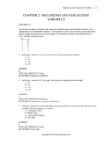
FIGURE 1–1 Mean, Median, and Mode for Example 1–2
Mode Median
(26.9)
Mean
18 20 22 24 26 28 30 32 34 36 38 40 42 44 46 48 50 52 54 56
x
When our observation set constitutes an entire population, instead of denoting the

mean by we use the symbol ␮ (the Greek letter mu). For a population, we use N as
the number of elements instead of n. The population mean is defined as follows.
x
Introduction and Descriptive Statistics 11
Mean of a population:
(1–2)
␮ =
a
N
i = 1
x
i
N
The mean of the observations in Example 1–2 is found as
= 538>20 = 26.9
+ 20 + 23 + 32 + 20 + 18)>20
+ 20 + 18 + 18 + 52 + 56 + 27 + 22 + 18 + 49 + 22
x = (x
1
+ x
2
+
###
+ x
20
)>20 = (33 + 26 + 24 + 21 + 19
The mean of the observations of Example 1–2, their average, is 26.9.
Figure 1–1 shows the data of Example 1–2 drawn on the number line along with
the mean, median, and mode of the observations. If you think of the data points as
little balls of equal weight located at the appropriate places on the number line, the

mean is that point where all the weights balance. It is the fulcrum of the point-weights,
as shown in Figure 1–1.
What characterizes the three measures of centrality, and what are the relative
merits of each? The mean summarizes all the information in the data. It is the aver-
age of all the observations. The mean is a single point that can be viewed as the point
where all the mass—the weight—of the observations is concentrated. It is the center of
mass of the data. If all the observations in our data set were the same size, then
(assuming the total is the same) each would be equal to the mean.
The median, on the other hand, is an observation (or a point between two obser-
vations) in the center of the data set. One-half of the data lie above this observation,
and one-half of the data lie below it. When we compute the median, we do not consider
the exact location of each data point on the number line; we only consider whether it
falls in the half lying above the median or in the half lying below the median.
What does this mean? If you look at the picture of the data set of Example 1–2,
Figure 1–1, you will note that the observation x
10
ϭ 56 lies to the far right. If we shift
this particular observation (or any other observation to the right of 22) to the right,
say, move it from 56 to 100, what will happen to the median? The answer is:
absolutely nothing (prove this to yourself by calculating the new median). The exact
location of any data point is not considered in the computation of the median, only
Aczel−Sounderpandian:
Complete Business
Statistics, Seventh Edition
1. Introduction and
Descriptive Statistics
Text
14
© The McGraw−Hill
Companies, 2009

its relative standing with respect to the central observation. The median is resistant to
extreme observations.
The mean, on the other hand, is sensitive to extreme observations. Let us see
what happens to the mean if we change x
10
from 56 to 100. The new mean is
12 Chapter 1
= 29.1

+ 22 + 18 + 49 + 22 + 20 + 23 + 32 + 20 + 18)>20
x
= (33 + 26 + 24 + 21 + 19 + 20 + 18 + 18 + 52 + 100 + 27
We see that the mean has shifted 2.2 units to the right to accommodate the change in
the single data point x
10
.
The mean, however, does have strong advantages as a measure of central ten-
dency. The mean is based on information contained in all the observations in the data set, rather
than being an observation lying “in the middle” of the set. The mean also has some
desirable mathematical properties that make it useful in many contexts of statistical
inference. In cases where we want to guard against the influence of a few outlying
observations (called outliers), however, we may prefer to use the median.
To continue with the condominium prices from Example 1–1, a larger sample of ask-
ing prices for two-bedroom units in Boston (numbers in thousand dollars, rounded to
the nearest thousand) is
789, 813, 980, 880, 650, 700, 2,990, 850, 690
What are the mean and the median? Interpret their meaning in this case.
EXAMPLE 1–4
Arranging the data from smallest to largest, we get
650, 690, 700, 789, 813, 850, 880, 980, 2,990

There are nine observations, so the median is the value in the middle, that is, in the
fifth position. That value is 813 thousand dollars.
To compute the mean, we add all data values and divide by 9, giving 1,038 thou-
sand dollars
—
that is, $1,038,000. Now notice some interesting facts. The value 2,990
is clearly an outlier. It lies far to the right, away from the rest of the data bunched
together in the 650–980 range.
In this case, the median is a very descriptive measure of this data set: it tells us
where our data (with the exception of the outlier) are located. The mean, on the other
hand, pays so much attention to the large observation 2,990 that it locates itself at
1,038, a value larger than our largest observation, except for the outlier. If our outlier
had been more like the rest of the data, say, 820 instead of 2,990, the mean would
have been 796.9. Notice that the median does not change and is still 813. This is so
because 820 is on the same side of the median as 2,990.
Sometimes an outlier is due to an error in recording the data. In such a case it
should be removed. Other times it is “out in left field” (actually, right field in this case)
for good reason.
As it turned out, the condominium with asking price of $2,990,000 was quite dif-
ferent from the rest of the two-bedroom units of roughly equal square footage and
location. This unit was located in a prestigious part of town (away from the other
units, geographically as well). It had a large whirlpool bath adjoining the master bed-
room; its floors were marble from the Greek island of Paros; all light fixtures and
faucets were gold-plated; the chandelier was Murano crystal. “This is not your aver-
age condominium,” the realtor said, inadvertently reflecting a purely statistical fact in
addition to the intended meaning of the expression.
Solution
Aczel−Sounderpandian:
Complete Business
Statistics, Seventh Edition

1. Introduction and
Descriptive Statistics
Text
15
© The McGraw−Hill
Companies, 2009
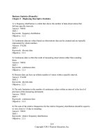
FIGURE 1–2 A Symmetrically Distributed Data Set
Mean = Median = Mode
x
1–18. Discuss the differences among the three measures of centrality.
1–19. Find the mean, median, and mode(s) of the observations in problem 1–13.
1–20. Do the same as problem 1–19, using the data of problem 1–14.
1–21. Do the same as problem 1–19, using the data of problem 1–15.
1–22. Do the same as problem 1–19, using the data of problem 1–16.
1–23. Do the same as problem 1–19, using the observation set in problem 1–17.
1–24. Do the same as problem 1–19 for the data in Example 1–1.
1–25. Find the mean, mode, and median for the data set 7, 8, 8, 12, 12, 12, 14, 15,
20, 47, 52, 54.
1–26. For the following stock price one-year percentage changes, plot the data and
identify any outliers. Find the mean and median.
6
Intel Ϫ6.9%
AT&T 46.5
General Electric 12.1
ExxonMobil 20.7
Microsoft 16.9
Pfizer 17.2
Citigroup 16.5
PROBLEMS
The mode tells us our data set’s most frequently occurring value. There may

be several modes. In Example 1–2, our data set actually possesses three modes:
18, 20, and 22. Of the three measures of central tendency, we are most interested
in the mean.
If a data set or population is symmetric (i.e., if one side of the distribution of the
observations is a mirror image of the other) and if the distribution of the observations
has only one mode, then the mode, the median, and the mean are all equal. Such a
situation is demonstrated in Figure 1–2. Generally, when the data distribution is
not symmetric, then the mean, median, and mode will not all be equal. The relative
positions of the three measures of centrality in such situations will be discussed in
section 1–6.
In the next section, we discuss measures of variability of a data set or population.
Introduction and Descriptive Statistics 13
6
“Stocks,” Money, March 2007, p. 128.
Aczel−Sounderpandian:
Complete Business
Statistics, Seventh Edition
1. Introduction and
Descriptive Statistics
Text
16
© The McGraw−Hill
Companies, 2009
FIGURE 1–3 Comparison of Data Sets I and II
x
Data are clustered together
45
6
78
Set II:

1
x
Data are spread out
2345
6
7891011
Set I:
Mean = Median = Mode = 6
Mean = Median = Mode = 6
1–27. The following data are the median returns on investment, in percent, for 10
industries.
7
Consumer staples 24.3%
Energy 23.3
Health care 22.1
Financials 21.0
Industrials 19.2
Consumer discretionary 19.0
Materials 18.1
Information technology 15.1
Telecommunication services 11.0
Utilities 10.4
Find the median of these medians and their mean.
1–4 Measures of Variability
Consider the following two data sets.
Set I: 1, 2, 3, 4, 5, 6, 6, 7, 8, 9, 10, 11
Set II: 4, 5, 5, 5, 6, 6, 6, 6, 7, 7, 7, 8
Compute the mean, median, and mode of each of the two data sets. As you see from your
results, the two data sets have the same mean, the same median, and the same mode,
all equal to 6. The two data sets also happen to have the same number of observations,

n ϭ 12. But the two data sets are different. What is the main difference between them?
Figure 1–3 shows data sets I and II. The two data sets have the same central ten-
dency (as measured by any of the three measures of centrality), but they have a dif-
ferent variability. In particular, we see that data set I is more variable than data set II.
The values in set I are more spread out: they lie farther away from their mean than
do those of set II.
There are several measures of variability, or dispersion. We have already dis-
cussed one such measure
—
the interquartile range. (Recall that the interquartile range
14 Chapter 1
7
“Sector Snapshot,” BusinessWeek, March 26, 2007, p. 62.
F
V
S
CHAPTER 1
Aczel−Sounderpandian:
Complete Business
Statistics, Seventh Edition
1. Introduction and
Descriptive Statistics
Text
17
© The McGraw−Hill
Companies, 2009
is defined as the difference between the upper quartile and the lower quartile.) The
interquartile range for data set I is 5.5, and the interquartile range of data set II is 2
(show this). The interquartile range is one measure of the dispersion or variability of
a set of observations. Another such measure is the range.

The range of a set of observations is the difference between the largest
observation and the smallest observation.
The range of the observations in Example 1–2 is Largest number Ϫ Smallest
number ϭ 56 Ϫ 18 ϭ 38. The range of the data in set I is 11 Ϫ 1 ϭ 10, and the range
of the data in set II is 8 Ϫ 4 ϭ 4. We see that, conforming with what we expect from
looking at the two data sets, the range of set I is greater than the range of set II. Set I is
more variable.
The range and the interquartile range are measures of the dispersion of a set of
observations, the interquartile range being more resistant to extreme observations.
There are also two other, more commonly used measures of dispersion. These are
the variance and the square root of the variance
—
the standard deviation.
The variance and the standard deviation are more useful than the range and the
interquartile range because, like the mean, they use the information contained in all
the observations in the data set or population. (The range contains information only on
the distance between the largest and smallest observations, and the interquartile range
contains information only about the difference between upper and lower quartiles.) We
define the variance as follows.
The variance of a set of observations is the average squared deviation of
the data points from their mean.
When our data constitute a sample, the variance is denoted by s
2
, and the aver-
aging is done by dividing the sum of the squared deviations from the mean by n Ϫ 1.
(The reason for this will become clear in Chapter 5.) When our observations consti-
tute an entire population, the variance is denoted by ␴
2
, and the averaging is done by
dividing by N. (And ␴ is the Greek letter sigma; we call the variance sigma squared.

The capital sigma is known to you as the symbol we use for summation, ⌺.)
Introduction and Descriptive Statistics 15
Sample variance:
(1–3)
s
2
=
a
n
i = 1
(x
i
- x)
2
n - 1
Population variance:
(1–4)
where ␮ is the population mean.
σ
2
ϭ
a
N
i ϭ 1
(x
i
Ϫ␮)
2
N
Recall that x

¯¯
is the sample mean, the average of all the observations in the sample.
Thus, the numerator in equation 1–3 is equal to the sum of the squared differences of
the data points x
i
(where i ϭ 1, 2, . . . , n) from their mean x
¯¯
. When we divide the
numerator by the denominator n Ϫ 1, we get a kind of average of the items summed
in the numerator. This average is based on the assumption that there are only n Ϫ 1
data points. (Note, however, that the summation in the numerator extends over all n
data points, not just n Ϫ 1 of them.) This will be explained in section 5–5.
When we have an entire population at hand, we denote the total number of
observations in the population by N. We define the population variance as follows.
Aczel−Sounderpandian:
Complete Business
Statistics, Seventh Edition
1. Introduction and
Descriptive Statistics
Text
18
© The McGraw−Hill
Companies, 2009
Unless noted otherwise, we will assume that all our data sets are samples and do
not constitute entire populations; thus, we will use equation 1–3 for the variance, and
not equation 1–4. We now define the standard deviation.
The standard deviation of a set of observations is the (positive) square
root of the variance of the set.
The standard deviation of a sample is the square root of the sample variance, and the
standard deviation of a population is the square root of the variance of the population.

8
16 Chapter 1
Sample standard deviation:
(1–5)s = 2s
2
=
H
a
n
i =1
(x
i
- x)
2
n - 1
Population standard deviation:
(1–6)␴ = 2␴
2
=
H
a
n
i =1
(x
i
- ␮)
2
n
- 1
Why would we use the standard deviation when we already have its square, the

variance? The standard deviation is a more meaningful measure. The variance is
the average squared deviation from the mean. It is squared because if we just compute
the deviations from the mean and then averaged them, we get zero (prove this with any
of the data sets). Therefore, when seeking a measure of the variation in a set of obser-
vations, we square the deviations from the mean; this removes the negative signs, and
thus the measure is not equal to zero. The measure we obtain
—
the variance
—
is still a
squared quantity; it is an average of squared numbers. By taking its square root, we
“unsquare” the units and get a quantity denoted in the original units of the problem
(e.g., dollars instead of dollars squared, which would have little meaning in most
applications). The variance tends to be large because it is in squared units. Statisti-
cians like to work with the variance because its mathematical properties simplify
computations. People applying statistics prefer to work with the standard deviation
because it is more easily interpreted.
Let us find the variance and the standard deviation of the data in Example 1–2.
We carry out hand computations of the variance by use of a table for convenience.
After doing the computation using equation 1–3, we will show a shortcut that will
help in the calculation. Table 1–3 shows how the mean is subtracted from each of
the values and the results are squared and added. At the bottom of the last column we
find the sum of all squared deviations from the mean. Finally, the sum is divided by
n Ϫ 1, giving s
2
, the sample variance. Taking the square root gives us s, the sample
standard deviation.
x
8
A note about calculators: If your calculator is designed to compute means and standard deviations, find the

key for the standard deviation. Typically, there will be two such keys. Consult your owner’s handbook to be sure you
are using the key that will produce the correct computation for a sample (division by n Ϫ 1) versus a population
(division by N ).
Aczel−Sounderpandian:
Complete Business
Statistics, Seventh Edition
1. Introduction and
Descriptive Statistics
Text
19
© The McGraw−Hill
Companies, 2009
By equation 1–3, the variance of the sample is equal to the sum of the third column
in the table, 2,657.8, divided by n Ϫ 1: s
2
ϭ 2,657.8͞19 ϭ 139.88421. The standard
deviation is the square root of the variance: s ϭ
ϭ 11.827266
, or, using
two-decimal accuracy,
9
s ϭ 11.83.
If you have a calculator with statistical capabilities, you may avoid having to use
a table such as Table 1–3. If you need to compute by hand, there is a shortcut formula
for computing the variance and the standard deviation.
1139.88421
Introduction and Descriptive Statistics 17
Shortcut formula for the sample variance:
(1–7)s
2

=
a
n
i = 1
x
2
i
- a
a
n
i = 1
x
i
b
2
n
n
n - 1
TABLE 1–3 Calculations Leading to the Sample Variance in Example 1–2
xxϪ (x Ϫ )
2
18 18 Ϫ 26.9 ϭϪ8.9 79.21
18 18 Ϫ 26.9 ϭϪ8.9 79.21
18 18 Ϫ 26.9 ϭϪ8.9 79.21
18 18 Ϫ 26.9 ϭϪ8.9 79.21
19 19 Ϫ 26.9 ϭϪ7.9 62.41
20 20 Ϫ 26.9 ϭϪ6.9 47.61
20 20 Ϫ 26.9 ϭϪ6.9 47.61
20 20 Ϫ 26.9 ϭϪ6.9 47.61
21 21 Ϫ 26.9 ϭϪ5.9 34.81

22 22 Ϫ 26.9 ϭϪ4.9 24.01
22 22 Ϫ 26.9 ϭϪ4.9 24.01
23 23 Ϫ 26.9 ϭϪ3.9 15.21
24 24 Ϫ 26.9 ϭϪ2.9 8.41
26 26 Ϫ 26.9 ϭϪ0.9 0.81
27 27 Ϫ 26.9 ϭ 0.1 0.01
32 32 Ϫ 26.9 ϭ 5.1 26.01
33 33 Ϫ 26.9 ϭ 6.1 37.21
49 49 Ϫ 26.9 ϭ 22.1 488.41
52 52 Ϫ 26.9 ϭ 25.1 630.01
56 56 Ϫ 26.9 ϭ 29.1 846.81
____ ________
0 2,657.8
xx
Again, the standard deviation is just the square root of the quantity in equation 1–7.
We will now demonstrate the use of this computationally simpler formula with the
data of Example 1–2. We will then use this simpler formula and compute the variance
and the standard deviation of the two data sets we are comparing: set I and set II.
As before, a table will be useful in carrying out the computations. The table for
finding the variance using equation 1–7 will have a column for the data points x and
9
In quantitative fields such as statistics, decimal accuracy is always a problem. How many digits after the decimal point
should we carry? This question has no easy answer; everything depends on the required level of accuracy. As a rule, we will
use only two decimals, since this suffices in most applications in this book. In some procedures, such as regression analysis,
more digits need to be used in computations (these computations, however, are usually done by computer).
Aczel−Sounderpandian:
Complete Business
Statistics, Seventh Edition
1. Introduction and
Descriptive Statistics

Text
20
© The McGraw−Hill
Companies, 2009
a column for the squared data points x
2
. Table 1–4 shows the computations for the
variance of the data in Example 1–2.
Using equation 1–7, we find
18 Chapter 1
= 139.88421
s
2
=
a
n
i= 1
x
2
i
- a
a
n
i= 1
x
i
b
2
n
n

n - 1
=
17,130 - (538)
2
>20
19
=
17,130 - 289,444>20
19
The standard deviation is obtained as before: s ϭϭ11.83. Using the
same procedure demonstrated with Table 1–4, we find the following quantities lead-
ing to the variance and the standard deviation of set I and of set II. Both are assumed
to be samples, not populations.
Set I: ⌺x ϭ 72, ⌺x
2
ϭ 542, s
2
ϭ 10, and s ϭϭ3.16
Set II: ⌺x ϭ 72, ⌺x
2
ϭ 446, s
2
ϭ 1.27, and s ϭϭ1.13
As expected, we see that the variance and the standard deviation of set II are smaller
than those of set I. While each has a mean of 6, set I is more variable. That is, the val-
ues in set I vary more about their mean than do those of set II, which are clustered
more closely together.
The sample standard deviation and the sample mean are very important statistics
used in inference about populations.
21.27

210
2139.88421
TABLE 1–4 Shortcut
Computations for the
Variance in Example 1–2
xx
2
18 324
18 324
18 324
18 324
19 361
20 400
20 400
20 400
21 441
22 484
22 484
23 529
24 576
26 676
27 729
32 1,024
33 1,089
49 2,401
52 2,704
56 3,136
538 17,130
In financial analysis, the standard deviation is often used as a measure of volatility and
of the risk associated with financial variables. The data below are exchange rate values

of the British pound, given as the value of one U.S. dollar’s worth in pounds. The first
column of 10 numbers is for a period in the beginning of 1995, and the second column
of 10 numbers is for a similar period in the beginning of 2007.
10
During which period,
of these two precise sets of 10 days each, was the value of the pound more volatile?
1995 2007
0.6332 0.5087
0.6254 0.5077
0.6286 0.5100
0.6359 0.5143
0.6336 0.5149
0.6427 0.5177
0.6209 0.5164
0.6214 0.5180
0.6204 0.5096
0.6325 0.5182
Solution
EXAMPLE 1–5
We are looking at two populations of 10 specific days at the start of each year (rather
than a random sample of days), so we will use the formula for the population standard
deviation. For the 1995 period we get ␴ϭ0.007033. For the 2007 period we get ␴ϭ
0.003938. We conclude that during the 1995 ten-day period the British pound was
10
From data reported in
“Business Day,” The New York Times, in March 2007, and from Web information.
Aczel−Sounderpandian:
Complete Business
Statistics, Seventh Edition
1. Introduction and

Descriptive Statistics
Text
21
© The McGraw−Hill
Companies, 2009
Introduction and Descriptive Statistics 19
The data for second quarter earnings per share (EPS) for major banks in the
Northeast are tabulated below. Compute the mean, the variance, and the standard
deviation of the data.
Name EPS
Bank of New York $2.53
Bank of America 4.38
Banker’s Trust/New York 7.53
Chase Manhattan 7.53
Citicorp 7.96
Brookline 4.35
MBNA 1.50
Mellon 2.75
Morgan JP 7.25
PNC Bank 3.11
Republic 7.44
State Street 2.04
Summit 3.25
EXAMPLE 1–6
Solution
s
2
= 5.94;

s = $2.44.

a
x = $61.62;

x = $4.74;

a
x
2
= 363.40;
FIGURE 1–4 Using Excel for Example 1–2
1
2
3
4
5
6
7
8
9
10
11
12
13
14
15
16
17
18
19
20

21
22
23
ABC D E FGH
Wealth ($billion)
33
26
24
21
20
19
18
18
52
56
27
22
18
49
22
20
23
32
20
18
Descriptive
Statistics
Mean
Median
Standard Deviation

Mode
Standard Error
Kurtosis
Skewness
Range
Minimum
Maximum
Sum
Count
Result
26.9
22
11.8272656
18
2.64465698
1.60368514
1.65371559
38
18
56
538
20
Excel Command
=AVERAGE(A3:A22)
=MEDIAN(A3:A22)
=STDEV(A3:A22)
=MODE(A3:A22)
=F11/SQRT(20)
=KURT(A3:A22)
=SKEW(A3:A22)

=MAX(A3:A22)-MIN(A3:A22)
=MIN(A3:A22)
=MAX(A3:A22)
=SUM(A3:A22)
=COUNT(A3:A22)
Figure 1–4 shows how Excel commands can be used for obtaining a group of the
most useful and common descriptive statistics using the data of Example 1–2. In sec-
tion 1–10, we will see how a complete set of descriptive statistics can be obtained
from a spreadsheet template.
more volatile than in the same period in 2007. Notice that if these had been random
samples of days, we would have used the sample standard deviation. In such cases we
might have been interested in statistical inference to some population.