BÀI GIẢNG KINH tế vĩ mô trương quang hùng
Bạn đang xem bản rút gọn của tài liệu. Xem và tải ngay bản đầy đủ của tài liệu tại đây (1.69 MB, 65 trang )
21/12/2011
1
Chapter 20
Introduction to macroeconomics
and national income accounting
David Begg, Stanley Fischer and Rudiger Dornbusch, Economics,
6th Edition, McGraw-Hill, 2000
Power Point presentation by Peter Smith
20.1
Macroeconomics is
the study of the economy as a whole
it deals with broad aggregates
but uses the same style of thinking
about economic issues as in
microeconomics.
20.2
Some key issues in macroeconomics
Inflation
– the rate of change of the general price level
Unemployment
– a measure of the number of people looking for
work, but who are without jobs
Output
– real gross national product (GNP) measures
total income of an economy
it is closely related to the economy's total output
thi UEH - dethiueh.com
www.facebook.com/dethi.ueh
21/12/2011
2
20.3
More key issues in macroeconomics
Economic growth
– increases in real GNP, an indication of
the expansion of the economy’s total
output
Macroeconomic policy
– a variety of policy measures used by
the government to affect the overall
performance of the economy
20.4
Inflation in the UK, 1950-99
0
5
10
15
20
25
30
195
0
19
70
19
90
% p.a.
Source: Economic Trends Annual Supplement, Labour Market Trends
20.5
Inflation in selected European countries
0 1 2 3 4 5
% change 1998 compared with 1997
Greece
Portugal
Italy
Spain
UK
Finland
EU
Belgium
France
Germany
thi UEH - dethiueh.com
www.facebook.com/dethi.ueh
21/12/2011
3
20.6
Inflation in UK, USA and Germany
0
2
4
6
8
10
12
14
16
% p.a.
1960-73 1973-81 1981-90 1990-98
UK USA Germany
20.7
Unemployment in the UK, 1950-99
0
2
4
6
8
10
12
14
195
0
19
70
19
90
% p.a.
Source: Economic Trends Annual Supplement, Labour Market Trends
20.8
Unemployment
in selected European countries
0 5 10 15 20
% unemployment (ILO measure) 1998
Greece
Portugal
Italy
Spain
UK
Finland
EU
Belgium
France
Germany
thi UEH - dethiueh.com
www.facebook.com/dethi.ueh
21/12/2011
4
20.9
Unemployment
in UK, USA and Germany
0
2
4
6
8
10
% p.a.
1960-73 1973-81 1981-90 1990-98
UK USA Germany
20.10
Economic growth
in UK, USA and Germany
0
1
2
3
4
5
% p.a.
1960-73 1973-81 1981-90 1990-98
UK USA Germany
20.11
The circular flow of income,
expenditure and output
Y
Households Firms
C + I
I
C
S
thi UEH - dethiueh.com
www.facebook.com/dethi.ueh
21/12/2011
5
20.12
Government in the circular flow
Y
C + I + G
I
C
S
Households FirmsGovernment
C + I + G - T
e
T
e
G
B - T
d
Y + B - T
d
20.13
Adding the foreign sector
To incorporate the foreign sector into
the circular flow
we must recognize that residents of a
country will buy imports from abroad
and that domestic firms will sell
(export) goods and services abroad.
20.14
GDP and GNP
Gross domestic product (GDP)
– measures the output produced by
factors of production located in the
domestic economy
Gross national product (GNP)
– measures the total income earned by
domestic citizens
GNP = GDP + net income from abroad
thi UEH - dethiueh.com
www.facebook.com/dethi.ueh
21/12/2011
6
20.15
Three measures of national output
Expenditure
– the sum of expenditures in the economy
– Y = C + I + G + X - Z
Income
– the sum of incomes paid for factor
services
– wages, profits, etc.
Output
– the sum of output (value added)
produced in the economy
20.16
National income accounting: a summary
GNP
(and
GNI)
at
market
prices
GDP
at
market
prices
NYA
C
X - Z
I
NYA
G
NNP
at basic
prices
Deprec'n
National
income
Indirect
taxes
Wages
and
salaries
Self-
employment
Profits,
rents
20.17
What GNP does and does not measure
Some care is needed:
– to distinguish between real and nominal
measurements
– to take account of population changes
– to remember that GNP is not a
comprehensive measure of everything
that contributes to economic welfare
thi UEH - dethiueh.com
www.facebook.com/dethi.ueh
21/12/201121/12/2011
11
Chapter 21
The determination of national income
David Begg, Stanley Fischer and Rudiger Dornbusch, Economics,
6th Edition, McGraw-Hill, 2000
Power Point presentation by Peter Smith
21.1
Aggregate output in the short run
Potential output
– the output the economy would produce
if all factors of production were fully
employed
Actual output
– what is actually produced in a period
– which may diverge from the potential
level
21.2
Some simplifying assumptions
Prices and wages are fixed
The actual quantity of total output is
demand-determined
– this will be a “Keynesian” model
For now, also assume:
– no government
– no foreign trade
Later chapters relax these assumptions
thi UEH - dethiueh.com
www.facebook.com/dethi.ueh
21/12/201121/12/2011
22
21.3
Aggregate demand
Given no government and no
international trade, aggregate
demand has two components:
– Investment
firms’ desired or planned additions to
physical capital & inventories
for now, assume this is autonomous
– Consumption
households’ demand for goods and services
so, AD = C + I
21.4
Consumption demand
Households allocate their income
between CONSUMPTION and
SAVING
Personal Disposable Income
– income that households have for
spending or saving
– income from their supply of factor
services (plus transfers less taxes)
21.5
Consumption and income in the UK
at constant 1995 prices, 1989-1998
350
375
400
425
450
475
500
400 425 450 475 500 525 550
Real disposable income (£bn.)
Household consumtpion
expenditure (£bn.)
Income is a strong influence on consumptionIncome is a strong influence on consumption
expenditure expenditure –– but not the only one.but not the only one.
thi UEH - dethiueh.com
www.facebook.com/dethi.ueh
21/12/201121/12/2011
33
21.6
The consumption function
IncomeIncome
C = 8 + 0.7 YC = 8 + 0.7 Y
The consumption function shows desired aggregateThe consumption function shows desired aggregate
consumption at each level of aggregate incomeconsumption at each level of aggregate income
00
With zero income,With zero income,
desired consumptiondesired consumption
is 8 (“autonomousis 8 (“autonomous
consumption”).consumption”).
{{
88
The The marginal propensitymarginal propensity
to consumeto consume (the slope of(the slope of
the function) is 0.7 the function) is 0.7 –– i.e.i.e.
for each additional £1 of for each additional £1 of
income, 70p is consumed.income, 70p is consumed.
21.7
The saving function
S = S = 8 + 0.3 Y8 + 0.3 Y
IncomeIncome
00
The saving function showsThe saving function shows
desired saving at eachdesired saving at each
income level.income level.
Since all income is either Since all income is either
saved or spent on saved or spent on
consumption, the savingconsumption, the saving
function can be derivedfunction can be derived
from the consumption from the consumption
function or function or vice versa.vice versa.
21.8
The aggregate demand schedule
IncomeIncome
CC
Aggregate demand isAggregate demand is
what households planwhat households plan
to spend on consumptionto spend on consumption
and what firms plan toand what firms plan to
spend on investment.spend on investment.
AD = C + IAD = C + I
II
The AD function is The AD function is
the vertical additionthe vertical addition
of C and I.of C and I.
(For now I is assumed (For now I is assumed
autonomous.)autonomous.)
thi UEH - dethiueh.com
www.facebook.com/dethi.ueh
21/12/201121/12/2011
44
21.9
Equilibrium output
Output, IncomeOutput, Income
4545
oo
lineline
The 45The 45
o o
line shows the line shows the
points at which desiredpoints at which desired
spending equals output spending equals output
or income.or income.
ADAD
Given the Given the ADAD schedule,schedule,
This the point at whichThis the point at which
planned spending equalsplanned spending equals
actual output and income.actual output and income.
equilibrium is thus at E.equilibrium is thus at E.
EE
21.10
An alternative approach
Output, IncomeOutput, Income
An equivalent view ofAn equivalent view of
equilibrium is seen byequilibrium is seen by
equatingequating
II
planned investment (planned investment (II))
SS
to planned saving (to planned saving (SS))
The two approaches are equivalent.The two approaches are equivalent.
again giving usagain giving us
equilibrium at Eequilibrium at E
EE
21.11
Effects of a fall in aggregate demand
Output, IncomeOutput, Income
4545
oo
lineline
ADAD
00
YY
00
Suppose the economySuppose the economy
starts in equilibrium starts in equilibrium
at Yat Y
0.0.
a fall in aggregate a fall in aggregate
demand to ADdemand to AD
11
ADAD
11
Leads the economyLeads the economy
to a new equilibrium to a new equilibrium
at Yat Y
11
YY
11
Notice that the change in equilibrium output isNotice that the change in equilibrium output is
larger than the original change in AD.larger than the original change in AD.
thi UEH - dethiueh.com
www.facebook.com/dethi.ueh
21/12/201121/12/2011
55
21.12
The multiplier
The multiplier is the ratio of the
change in equilibrium output to the
change in autonomous spending that
causes the change in output.
The larger the marginal propensity to
consume, the larger is the multiplier.
– The higher is the marginal propensity to
save, the more of each extra unit of
income “leaks” out of the circular flow.
thi UEH - dethiueh.com
www.facebook.com/dethi.ueh
21/12/2011
1
Chapter 22
Aggregate demand, fiscal policy,
and foreign trade
David Begg, Stanley Fischer and Rudiger Dornbusch, Economics,
6th Edition, McGraw-Hill, 2000
Power Point presentation by Peter Smith
22.1
Some key terms
Fiscal policy
– the government’s decisions about spending
and taxes
Stabilization policy
– government actions to try to keep output close
to its potential level
Budget deficit
– the excess of government outlays over
government receipts
National debt
– the stock of outstanding government debt
22.2
Government
in the income-expenditure model
Direct taxes
– affect the slope of the consumption
function
– and hence the slope of the AD
schedule.
Government expenditure affects the
position of the AD schedule
thi UEH - dethiueh.com
www.facebook.com/dethi.ueh
21/12/2011
2
22.3
Fiscal policy?
Income,
output
45
o
line
AD
0
Y
0
But this ignores some
important issues –
prices, interest rates,
and the need to fund
the government
spending.
AD
1
This seems to suggest
that the government
could influence aggregate
output in the economy
by raising AD from AD
0
to AD
1
,
Y
1
thus raising equilibrium
output from Y
0
to Y
1
.
22.4
but in surplus at high levels
then the budget will be in
deficit at low levels of
income
The government budget
The budget deficit equals total government spending
minus total tax revenue.
If government spending is
independent of income
G
Income, output
but net taxes depend on
income,
The balanced budget multiplier states that an increase in
government spending plus an equal increase in taxes leads
to higher equilibrium output.
Balanced
budget
22.5
Deficits and the fiscal stance
The size of the budget deficit is not a good
measure of the government’s fiscal
stance.
The structural budget shows what the
budget would have been if output had
been at the full-employment level.
The inflation-adjusted budget uses real
not nominal interest rates to calculate
government spending on debt interest.
thi UEH - dethiueh.com
www.facebook.com/dethi.ueh
21/12/2011
3
22.6
Automatic stabilizers
mechanisms in the economy that
reduce the response of GNP to
shocks
– for example, in a recession:
– payments of unemployment benefits
rise
– and receipts from VAT and income tax
fall
22.7
Limits on active fiscal policy
Time lags: it takes time
– to diagnose the problem
– to take action
– for the multiplier process to operate
Uncertainty
– the size of the multiplier is not known
– aggregate demand is always changing
Induced effects on autonomous demand
– changes in fiscal policy may induce offsetting effects in
other components of aggregate demand
Why can’t shocks to aggregate demand
immediately be offset by fiscal policy?
22.8
Limits on active fiscal policy (2)
The budget deficit
– concern about inflation if the budget deficit
grows
Maybe we’re at full employment!
– unemployment may be (at least partly)
voluntary
Why doesn’t the government expand fiscal
policy when unemployment is persistently high?
thi UEH - dethiueh.com
www.facebook.com/dethi.ueh
21/12/2011
4
22.9
Foreign trade
and income determination
Introducing exports (X) & imports (Z)
TRADE BALANCE
– the value of net exports (X - Z)
TRADE DEFICIT
– when imports exceed exports
TRADE SURPLUS
– when exports exceed imports
Equilibrium is now where
– Y = C + I + G + X - Z
22.10
At higher income levels, there is a trade deficit.
At relatively low income,
exports exceed imports – there is a trade surplus.
Exports, imports and the trade balance
Income
but that imports increase
with income
Imports
Assume that exports
are independent of
income,
Exports
There is trade balance at income Y*, but there is no
guarantee that this corresponds to full employment.
Y*
22.11
Foreign trade and the multiplier
The marginal propensity to import
– is the fraction of additional income that
domestic residents wish to spend on
additional imports.
The effect of foreign trade is to
reduce the size of the multiplier
– the higher the value of the marginal
propensity to import, the lower the
value of the multiplier.
thi UEH - dethiueh.com
www.facebook.com/dethi.ueh
21/12/2011
1
Chapter 23
Money and modern banking
David Begg, Stanley Fischer and Rudiger Dornbusch, Economics,
6th Edition, McGraw-Hill, 2000
Power Point presentation by Peter Smith
23.1
Some key questions
Why does society need money?
Why do governments wish to
influence money supply?
How do financial markets interact
with the “real” economy?
What is the relationship between
money and interest rates?
23.2
Money
Any generally accepted means of
payment for delivery of goods or the
settlement of debt
Legal money
– notes and coins
Customary money
– IOU money based on private debt of the
individual
e.g. bank deposit.
thi UEH - dethiueh.com
www.facebook.com/dethi.ueh
21/12/2011
2
23.3
Money and its functions
Medium of exchange
– money provides a medium for the exchange of goods
and services which is more efficient than barter
Unit of account
– a unit in which prices are quoted and accounts are kept
Store of value
– money can be used to make purchases in the future
Standard of deferred payment
– a unit of account over time: this enables borrowing and
lending
23.4
Modern banking
A financial intermediary
– an institution that specializes in bringing
lenders and borrowers together
e.g. a commercial bank, which has a government
licence to make loans and issue deposits
including deposits against which cheques can be
written
Clearing system
– a set of arrangements in which debts between
banks are settled
23.5
A beginner’s guide to the financial markets
Financial asset
– a piece of paper entitling the owner to a
specified stream of interest payments over a
specified period
Cash
– Notes and coin, paying no interest
– the most liquid of all assets.
Bills
– financial assets with less than one year until
the known date at which they will be
repurchased by the original owner
– highly liquid
thi UEH - dethiueh.com
www.facebook.com/dethi.ueh
21/12/2011
3
23.6
A beginner’s guide to the financial markets
(continued)
Bonds
– longer term financial assets – less liquid because there
is more uncertainty about the future income stream
Perpetuities
– an extreme form of bond, never repurchased by the
original issuer, who pays interest forever
e.g. Consols
Gilt-edged securities
– government bonds in the UK
Industrial shares (equities)
– entitlements to receive corporate dividends
– not very liquid
23.7
Credit creation by banks
Commercial banks need to hold only
a proportion of assets as cash
reserves
– this enables them to create credit by
lending
EXAMPLE:
– suppose the public needs a fixed £10m
for transactions
– and the commercial bank maintains a
10% cash reserve
23.8
Credit creation – example
Commercial bank :
Liabilities
Assets
Deposits
Cash Loans Total
Cash
ratio
%
Public
cash
holding
Money
supply
Initial position:
100 10 90 100
Central bank issues £10m extra; the public deposits it
10
10
110
110 20 90 110
1
18.2 10 120
110 11 99 1102 10 19 129
119 20 99 1193 16.8 10 129
200 20 180 200
n
10 10 210
thi UEH - dethiueh.com
www.facebook.com/dethi.ueh
21/12/2011
4
23.9
The monetary base and the
money multiplier
The monetary base or stock of high-
powered money
– the quantity of notes and coin in private
circulation plus the quantity held by the
banking system
The money multiplier
– the change in the money stock for a £1
change in the quantity of the monetary
base
23.10
The money multiplier
Suppose the banks wish to hold cash reserves R as
as fraction (c
b
) of deposits (D), and the private sector
wish to hold cash (C) as a fraction (c
p
) of bank
deposits (D).
Then R = c
b
D and C = c
p
D
Monetary base H = C + R = (c
b
+ c
p
) D
Money supply = C + D = (c
p
+ 1) D
So M =
(c
p
+ 1)
(c
p
+ c
b
)
H
Money supply = money multiplier × monetary base
thi UEH - dethiueh.com
www.facebook.com/dethi.ueh
21/12/2011
1
Chapter 24
Central banking and the
monetary system
David Begg, Stanley Fischer and Rudiger Dornbusch, Economics,
6th Edition, McGraw-Hill, 2000
Power Point presentation by Peter Smith
24.1
The central bank
acts as banker to the commercial
banks in a country
and is responsible for setting interest
rates.
In the UK, the Bank of England fulfils
these roles.
Two key tasks:
– to issue coins and bank-notes
– to act as banker to the banking system
and the government.
24.2
The Bank and the money supply
Three ways in which the central bank MAY
influence money supply:
– Reserve requirements
central bank sets a minimum ratio of cash reserves
to deposits that commercial banks must meet
– Discount rate
the interest rate that the central bank charges when
the commercial banks want to borrow
setting this at a penalty rate may encourage
commercial banks to hold more excess reserves
– Open market operations
actions to alter the monetary base by buying or
selling financial securities in the open market
thi UEH - dethiueh.com
www.facebook.com/dethi.ueh
21/12/2011
2
24.3
The repo market
A gilt repo is a sale and repurchase
agreement
– e.g. a bank sells you a gilt with a simultaneous
agreement to buy it back at a specified price at
a specified future date.
– this uses the outstanding stock of long-term
assets (gilts) as backing for new short-term
loans
Used by the Bank of England in carrying
out open market operations
24.4
Other functions of the Bank of England
Lender of last resort
– the Bank stands ready to lend to banks and
other financial institutions when financial
panic threatens
Banker to the government
– the Bank ensures that the government can
meet its payments when running a budget
deficit
Setting monetary policy to control
inflation
– more of this later
24.5
The demand for money
The opportunity cost of holding
money is the interest given up by
holding money rather than bonds.
People will only hold money if there
is a benefit to offset that opportunity
cost.
thi UEH - dethiueh.com
www.facebook.com/dethi.ueh
21/12/2011
3
24.6
Motives for holding money
Transactions
– payments and receipts are not perfectly
synchronized:
so money is held to finance known transactions
depends upon income and payment arrangements
Precautionary
– because of uncertainty:
people hold money to meet unforeseen
contingencies
depends upon the (nominal) interest rate
24.7
Motives for holding money (2)
Asset
– people dislike risk
– so may hold money as a low-risk component
of a mixed portfolio
depends upon opportunity cost (the nominal interest
rate)
Speculative
– people may hold money rather than bonds
– if bond prices are expected to fall
– i.e. the interest rate is expected to rise
depends upon the rate of interest and on
expectations about bond prices
24.8
The demand for money: summary
The demand for money is a demand
for real money balances
It depends upon:
– real income
– nominal interest rate (the opportunity
cost of holding money)
– the price level (currently assumed fixed)
– expectations about future interest rates
thi UEH - dethiueh.com
www.facebook.com/dethi.ueh
21/12/2011
4
24.9
Money market equilibrium
Real money holdings
LL
Other things being equal,
the demand for real money
balances will be lower when
the opportunity cost (the rate
of interest) is relatively high.
The position of this
schedule depends upon
real income and the price
level.
When money supply is L
0
, money market equilibrium
occurs when the rate of interest is at r
0
.
L
0
r
0
24.10
Reaching money market equilibrium
Real money holdings
LL
L
0
r
0
If the rate of interest is
set below the market
equilibrium – say at r
1
r
1
there is excess demand for
money (the distance
AB)
A B
This implies an excess
supply of bonds
– which reduces the price
of bonds
and thus raises the rate of interest until equilibrium
is reached.
24.11
Monetary control
Real money holdings
LL
L
0
r
0
Given the money demand schedule:
The central bank can
EITHER set the interest
rate at r
0
and allow money
supply to adjust to L
0
OR set money supply at L
0
and allow the market rate
of interest adjust to r
0
BUT cannot set both
money supply and interest
rate independently.
thi UEH - dethiueh.com
www.facebook.com/dethi.ueh
21/12/2011
5
24.12
Monetary control – some provisos
Monetary control cannot be precise unless
the authorities know the shape and
position of money demand
Controlling money supply is especially
problematic
– and the Bank of England has preferred to work
via interest rates
The situation is further complicated by the
relationship between the interest rate and
the exchange rate
24.13
Targets and instruments of
monetary policy
Monetary instrument:
– the variable over which the central bank
exercises day to day control
– e.g. interest rate
Intermediate target
– the key indicator used as an input to frequent
decisions about when to set interest rates
The financial revolution has reduced the
reliability of money supply as an indicator
– and central banks increasingly use inflation
forecasts as the intermediate target
thi UEH - dethiueh.com
www.facebook.com/dethi.ueh
21/12/2011
1
Chapter 25
Monetary and fiscal policy in a
closed economy
David Begg, Stanley Fischer and Rudiger Dornbusch, Economics,
6th Edition, McGraw-Hill, 2000
Power Point presentation by Peter Smith
25.1
Bringing together the real and financial sectors
Having seen equilibrium in the goods
and money markets separately,
it is now time to explore the links
between them
and to look at simultaneous
equilibrium in both.
25.2
Consumption revisited
Income is a key determinant of
consumption
but other factors shift the consumption
function
– household wealth
– availability of credit
– cost of credit
These create a link between the financial
and real sectors
– because interest rates can be seen to influence
consumption.
thi UEH - dethiueh.com
www.facebook.com/dethi.ueh