programming with matlab ebook
Bạn đang xem bản rút gọn của tài liệu. Xem và tải ngay bản đầy đủ của tài liệu tại đây (1.05 MB, 40 trang )
3
Programming with MATLAB
48
CHAPTER OBJECTIVES
The primary objective of this chapter is to learn how to write M-file programs to
implement numerical methods. Specific objectives and topics covered are
•
Learning how to create well-documented M-files in the edit window and invoke
them from the command window.
•
Understanding how script and function files differ.
•
Understanding how to incorporate help comments in functions.
•
Knowing how to set up M-files so that they interactively prompt users for
information and display results in the command window.
•
Understanding the role of subfunctions and how they are accessed.
•
Knowing how to create and retrieve data files.
•
Learning how to write clear and well-documented M-files by employing
structured programming constructs to implement logic and repetition.
•
Recognizing the difference between if elseif and switch constructs.
•
Recognizing the difference between for end and while structures.
•
Knowing how to animate MATLAB plots.
•
Understanding what is meant by vectorization and why it is beneficial.
•
Understanding how anonymous functions can be employed to pass functions to
function function M-files.
YOU’VE GOT A PROBLEM
I
n Chap. 1, we used a force balance to develop a mathematical model to predict the
fall velocity of a bungee jumper. This model took the form of the following differential
equation:
dv
dt
= g −
c
d
m
v|v|
cha01102_ch03_048-087.qxd 11/9/10 11:13 AM Page 48
CONFIRMING PAGES
We also learned that a numerical solution of this equation could be obtained with Euler’s
method:
v
i+1
= v
i
+
dv
i
dt
t
This equation can be implemented repeatedly to compute velocity as a function of
time. However, to obtain good accuracy, many small steps must be taken. This would be
extremely laborious and time consuming to implement by hand. However, with the aid of
MATLAB, such calculations can be performed easily.
So our problem now is to figure out how to do this. This chapter will introduce you to
how MATLAB M-files can be used to obtain such solutions.
3.1 M-FILES
The most common way to operate MATLAB is by entering commands one at a time in the
command window. M-files provide an alternative way of performing operations that
greatly expand MATLAB’s problem-solving capabilities. An M-file consists of a series of
statements that can be run all at once. Note that the nomenclature “M-file” comes from the
fact that such files are stored with a
.m extension. M-files come in two flavors: script files
and function files.
3.1.1 Script Files
A script file is merely a series of MATLAB commands that are saved on a file. They are
useful for retaining a series of commands that you want to execute on more than one occa-
sion. The script can be executed by typing the file name in the command window or by
invoking the menu selections in the edit window:
Debug, Run.
EXAMPLE 3.1 Script File
Problem Statement. Develop a script file to compute the velocity of the free-falling
bungee jumper for the case where the initial velocity is zero.
Solution. Open the editor with the menu selection:
File, New, M-file. Type in the follow-
ing statements to compute the velocity of the free-falling bungee jumper at a specific time
[recall Eq. (1.9)]:
g = 9.81; m = 68.1; t = 12; cd = 0.25;
v = sqrt(g * m / cd) * tanh(sqrt(g * cd / m) * t)
Save the file as scriptdemo.m. Return to the command window and type
>>scriptdemo
The result will be displayed as
v =
50.6175
Thus, the script executes just as if you had typed each of its lines in the command window.
3.1 M-FILES 49
cha01102_ch03_048-087.qxd 11/9/10 11:13 AM Page 49
CONFIRMING PAGES
As a final step, determine the value of g by typing
>> g
g =
9.8100
So you can see that even though g was defined within the script, it retains its value back in
the command workspace. As we will see in the following section, this is an important dis-
tinction between scripts and functions.
3.1.2 Function Files
Function files are M-files that start with the word function. In contrast to script files, they
can accept input arguments and return outputs. Hence they are analogous to user-defined
functions in programming languages such as Fortran, Visual Basic or C.
The syntax for the function file can be represented generally as
function outvar = funcname(arglist)
% helpcomments
statements
outvar = value;
where outvar = the name of the output variable, funcname = the function’s name,
arglist = the function’s argument list (i.e., comma-delimited values that are passed into
the function), helpcomments = text that provides the user with information regarding the
function (these can be invoked by typing Help funcname in the command window), and
statements = MATLAB statements that compute the value that is assigned to outvar.
Beyond its role in describing the function, the first line of the helpcomments, called
the H1 line, is the line that is searched by the lookfor command (recall Sec. 2.6). Thus,
you should include key descriptive words related to the file on this line.
The M-file should be saved as funcname.m. The function can then be run by typing
funcname in the command window as illustrated in the following example. Note that even
though MATLAB is case-sensitive, your computer’s operating system may not be.
Whereas MATLAB would treat function names like
freefall and FreeFall as two dif-
ferent variables, your operating system might not.
EXAMPLE 3.2 Function File
Problem Statement. As in Example 3.1, compute the velocity of the free-falling bungee
jumper but now use a function file for the task.
Solution. Type the following statements in the file editor:
function v = freefall(t, m, cd)
% freefall: bungee velocity with second-order drag
% v=freefall(t,m,cd) computes the free-fall velocity
% of an object with second-order drag
% input:
50 PROGRAMMING WITH MATLAB
cha01102_ch03_048-087.qxd 11/9/10 11:13 AM Page 50
CONFIRMING PAGES
% t = time (s)
% m = mass (kg)
% cd = second-order drag coefficient (kg/m)
% output:
% v = downward velocity (m/s)
g = 9.81; % acceleration of gravity
v = sqrt(g * m / cd)*tanh(sqrt(g * cd / m) * t);
Save the file as freefall.m. To invoke the function, return to the command window and
type in
>> freefall(12,68.1,0.25)
The result will be displayed as
ans =
50.6175
One advantage of a function M-file is that it can be invoked repeatedly for different
argument values. Suppose that you wanted to compute the velocity of a 100-kg jumper
after 8 s:
>> freefall(8,100,0.25)
ans =
53.1878
To invoke the help comments type
>> help freefall
which results in the comments being displayed
freefall: bungee velocity with second-order drag
v=freefall(t,m,cd) computes the free-fall velocity
of an object with second-order drag
input:
t = time (s)
m = mass (kg)
cd = second-order drag coefficient (kg/m)
output:
v = downward velocity (m/s)
If at a later date, you forgot the name of this function, but remembered that it involved
bungee jumping, you could enter
>> lookfor bungee
and the following information would be displayed
freefall.m - bungee velocity with second-order drag
Note that, at the end of the previous example, if we had typed
>> g
3.1 M-FILES 51
cha01102_ch03_048-087.qxd 11/9/10 11:13 AM Page 51
CONFIRMING PAGES
the following message would have been displayed
??? Undefined function or variable 'g'.
So even though g had a value of 9.81 within the M-file, it would not have a value in the
command workspace. As noted previously at the end of Example 3.1, this is an important
distinction between functions and scripts. The variables within a function are said to be
local and are erased after the function is executed. In contrast, the variables in a script
retain their existence after the script is executed.
Function M-files can return more than one result. In such cases, the variables contain-
ing the results are comma-delimited and enclosed in brackets. For example, the following
function, stats.m, computes the mean and the standard deviation of a vector:
function [mean, stdev] = stats(x)
n = length(x);
mean = sum(x)/n;
stdev = sqrt(sum((x-mean).^2/(n-1)));
Here is an example of how it can be applied:
>> y = [8 5 10 12 6 7.5 4];
>> [m,s] = stats(y)
m =
7.5000
s =
2.8137
Although we will also make use of script M-files, function M-files will be our primary
programming tool for the remainder of this book. Hence, we will often refer to function
M-files as simply M-files.
3.1.3 Subfunctions
Functions can call other functions. Although such functions can exist as separate M-files,
they may also be contained in a single M-file. For example, the M-file in Example 3.2
(without comments) could have been split into two functions and saved as a single
M-file
1
:
function v = freefallsubfunc(t, m, cd)
v = vel(t, m, cd);
end
function v = vel(t, m, cd)
g = 9.81;
v = sqrt(g * m / cd)*tanh(sqrt(g * cd / m) * t);
end
52 PROGRAMMING WITH MATLAB
1
Note that although end statements are not used to terminate single-function M-files, they are included when
subfunctions are involved to demarcate the boundaries between the main function and the subfunctions.
cha01102_ch03_048-087.qxd 11/9/10 11:13 AM Page 52
CONFIRMING PAGES
This M-file would be saved as freefallsubfunc.m. In such cases, the first function is
called the main or primary function. It is the only function that is accessible to the com-
mand window and other functions and scripts. All the other functions (in this case,
vel) are
referred to as subfunctions.
A subfunction is only accessible to the main function and other subfunctions within
the M-file in which it resides. If we run freefallsubfunc from the command window,
the result is identical to Example 3.2:
>> freefallsubfunc(12,68.1,0.25)
ans =
50.6175
However, if we attempt to run the subfunction vel, an error message occurs:
>> vel(12,68.1,.25)
??? Undefined function or method 'vel' for input arguments
of type 'double'.
3.2 INPUT-OUTPUT
As in Section 3.1, information is passed into the function via the argument list and is out-
put via the function’s name. Two other functions provide ways to enter and display infor-
mation directly using the command window.
The
input Function. This function allows you to prompt the user for values directly
from the command window. Its syntax is
n = input('promptstring')
The function displays the promptstring, waits for keyboard input, and then returns the
value from the keyboard. For example,
m = input('Mass (kg): ')
When this line is executed, the user is prompted with the message
Mass (kg):
If the user enters a value, it would then be assigned to the variable m.
The input function can also return user input as a string. To do this, an 's' is ap-
pended to the function’s argument list. For example,
name = input('Enter your name: ','s')
The disp Function. This function provides a handy way to display a value. Its syntax is
disp(value)
where value = the value you would like to display. It can be a numeric constant or vari-
able, or a string message enclosed in hyphens. Its application is illustrated in the following
example.
3.2 INPUT-OUTPUT 53
cha01102_ch03_048-087.qxd 11/9/10 11:13 AM Page 53
CONFIRMING PAGES
EXAMPLE 3.3 An Interactive M-File Function
Problem Statement. As in Example 3.2, compute the velocity of the free-falling bungee
jumper, but now use the
input and disp functions for input/output.
Solution. Type the following statements in the file editor:
function freefalli
% freefalli: interactive bungee velocity
% freefalli interactive computation of the
% free-fall velocity of an object
% with second-order drag.
g = 9.81; % acceleration of gravity
m = input('Mass (kg): ');
cd = input('Drag coefficient (kg/m): ');
t = input('Time (s): ');
disp(' ')
disp('Velocity (m/s):')
disp(sqrt(g * m / cd)*tanh(sqrt(g * cd / m) * t))
Save the file as freefalli.m. To invoke the function, return to the command window and
type
>> freefalli
Mass (kg): 68.1
Drag coefficient (kg/m): 0.25
Time (s): 12
Velocity (m/s):
50.6175
The fprintf Function. This function provides additional control over the display of
information. A simple representation of its syntax is
fprintf('format', x, )
where format is a string specifying how you want the value of the variable x to be dis-
played. The operation of this function is best illustrated by examples.
A simple example would be to display a value along with a message. For instance, sup-
pose that the variable velocity has a value of 50.6175. To display the value using eight
digits with four digits to the right of the decimal point along with a message, the statement
along with the resulting output would be
>> fprintf('The velocity is %8.4f m/s\n', velocity)
The velocity is 50.6175 m/s
This example should make it clear how the format string works. MATLAB starts at
the left end of the string and displays the labels until it detects one of the symbols: % or \.
In our example, it first encounters a % and recognizes that the following text is a format
code. As in Table 3.1, the format codes allow you to specify whether numeric values are
54 PROGRAMMING WITH MATLAB
cha01102_ch03_048-087.qxd 11/9/10 11:13 AM Page 54
CONFIRMING PAGES
displayed in integer, decimal, or scientific format. After displaying the value of velocity,
MATLAB continues displaying the character information (in our case the units: m/s) until
it detects the symbol \. This tells MATLAB that the following text is a control code. As in
Table 3.1, the control codes provide a means to perform actions such as skipping to the
next line. If we had omitted the code \n in the previous example, the command prompt
would appear at the end of the label m/s rather than on the next line as would typically be
desired.
The fprintf function can also be used to display several values per line with differ-
ent formats. For example,
>> fprintf('%5d %10.3f %8.5e\n',100,2*pi,pi);
100 6.283 3.14159e+000
It can also be used to display vectors and matrices. Here is an M-file that enters two
sets of values as vectors. These vectors are then combined into a matrix, which is then dis-
played as a table with headings:
function fprintfdemo
x = [1 2 3 4 5];
y = [20.4 12.6 17.8 88.7 120.4];
z = [x;y];
fprintf(' x y\n');
fprintf('%5d %10.3f\n',z);
The result of running this M-file is
>> fprintfdemo
x y
1 20.400
2 12.600
3 17.800
4 88.700
5 120.400
3.2 INPUT-OUTPUT 55
TABLE 3.1 Commonly used format and control codes employed
with the fprintf function.
Format Code Description
%d Integer format
%e Scientific format with lowercase e
%E Scientific format with uppercase E
%f Decimal format
%g The more compact of %e or %f
Control Code Description
\n Start new line
\t Tab
cha01102_ch03_048-087.qxd 11/9/10 11:13 AM Page 55
CONFIRMING PAGES
3.2.1 Creating and Accessing Files
MATLAB has the capability to both read and write data files. The simplest approach in-
volves a special type of binary file, called a MAT-file, which is expressly designed for
implementation within MATLAB. Such files are created and accessed with the save and
load commands.
The save command can be used to generate a MAT-file holding either the entire work-
space or a few selected variables. A simple representation of its syntax is
save filename var1 var2 varn
This command creates a MAT-file named filename.mat that holds the variables var1
through varn. If the variables are omitted, all the workspace variables are saved. The load
command can subsequently be used to retrieve the file:
load filename var1 var2 varn
which retrieves the variables var1 through varn from filename.mat. As was the case
with save, if the variables are omitted, all the variables are retrieved.
For example, suppose that you use Eq. (1.9) to generate velocities for a set of drag
coefficients:
>> g=9.81;m=80;t=5;
>> cd=[.25 .267 .245 .28 .273]';
>> v=sqrt(g*m ./cd).*tanh(sqrt(g*cd/m)*t);
You can then create a file holding the values of the drag coefficients and the velocities with
>> save veldrag v cd
To illustrate how the values can be retrieved at a later time, remove all variables from
the workspace with the clear command,
>> clear
At this point, if you tried to display the velocities you would get the result:
>> v
??? Undefined function or variable 'v'.
However, you can recover them by entering
>> load veldrag
Now, the velocities are available as can be verified by typing
>> who
Your variables are:
cd v
Although MAT-files are quite useful when working exclusively within the MATLAB
environment, a somewhat different approach is required when interfacing MATLAB with
other programs. In such cases, a simple approach is to create text files written in ASCII
format.
56 PROGRAMMING WITH MATLAB
cha01102_ch03_048-087.qxd 11/9/10 11:13 AM Page 56
CONFIRMING PAGES
ASCII files can be generated in MATLAB by appending –ascii to the save com-
mand. In contrast to MAT-files where you might want to save the entire workspace, you
would typically save a single rectangular matrix of values. For example,
>> A=[5 7 9 2;3 6 3 9];
>> save simpmatrix.txt –ascii
In this case, the save command stores the values in A in 8-digit ASCII form. If you want
to store the numbers in double precision, just append –ascii –double. In either case, the
file can be accessed by other programs such as spreadsheets or word processors. For
example, if you open this file with a text editor, you will see
5.0000000e+000 7.0000000e+000 9.0000000e+000 2.0000000e+000
3.0000000e+000 6.0000000e+000 3.0000000e+000 9.0000000e+000
Alternatively, you can read the values back into MATLAB with the load command,
>> load simpmatrix.txt
Because simpmatrix.txt is not a MAT-file, MATLAB creates a double precision array
named after the filename:
>> simpmatrix
simpmatrix =
5 7 9 2
3 6 3 9
Alternatively, you could use the load command as a function and assign its values to a
variable as in
>> A = load('simpmatrix.txt')
The foregoing material covers but a small portion of MATLAB’s file management ca-
pabilities. For example, a handy import wizard can be invoked with the menu selections:
File, Import Data. As an exercise, you can demonstrate the import wizards convenience by
using it to open simpmatrix.txt. In addition, you can always consult help to learn more
about this and other features.
3.3 STRUCTURED PROGRAMMING
The simplest of all M-files perform instructions sequentially. That is, the program state-
ments are executed line by line starting at the top of the function and moving down to the
end. Because a strict sequence is highly limiting, all computer languages include state-
ments allowing programs to take nonsequential paths. These can be classified as
• Decisions (or Selection). The branching of flow based on a decision.
• Loops (or Repetition). The looping of flow to allow statements to be repeated.
3.3.1 Decisions
The
if Structure. This structure allows you to execute a set of statements if a logical
condition is true. Its general syntax is
if condition
statements
end
3.3 STRUCTURED PROGRAMMING 57
cha01102_ch03_048-087.qxd 11/9/10 11:13 AM Page 57
CONFIRMING PAGES
where condition is a logical expression that is either true or false. For example, here is a
simple M-file to evaluate whether a grade is passing:
function grader(grade)
% grader(grade):
% determines whether grade is passing
% input:
% grade = numerical value of grade (0-100)
% output:
% displayed message
if grade >= 60
disp('passing grade')
end
The following illustrates the result
>> grader(95.6)
passing grade
For cases where only one statement is executed, it is often convenient to implement
the if structure as a single line,
if grade > 60, disp('passing grade'), end
This structure is called a single-line if. For cases where more than one statement is
implemented, the multiline if structure is usually preferable because it is easier to
read.
Error Function. A nice example of the utility of a single-line if is to employ it for rudi-
mentary error trapping. This involves using the
error function which has the syntax,
error(msg)
When this function is encountered, it displays the text message msg, indicates where
the error occurred, and causes the M-file to terminate and return to the command
window.
An example of its use would be where we might want to terminate an M-file to avoid
a division by zero. The following M-file illustrates how this could be done:
function f = errortest(x)
if x == 0, error('zero value encountered'), end
f = 1/x;
If a nonzero argument is used, the division would be implemented successfully as in
>> errortest(10)
ans =
0.1000
However, for a zero argument, the function would terminate prior to the division and the
error message would be displayed in red typeface:
>> errortest(0)
??? Error using ==> errortest at 2
zero value encountered
58 PROGRAMMING WITH MATLAB
cha01102_ch03_048-087.qxd 11/9/10 11:13 AM Page 58
CONFIRMING PAGES
Logical Conditions. The simplest form of the condition is a single relational expres-
sion that compares two values as in
value
1
relation value
2
where the values can be constants, variables, or expressions and the relation is one of
the relational operators listed in Table 3.2.
MATLAB also allows testing of more than one logical condition by employing logical
operators. We will emphasize the following:
•
~ (Not). Used to perform logical negation on an expression.
~expression
If the expression is true, the result is false. Conversely, if the expression is false,
the result is true.
• & (And ). Used to perform a logical conjunction on two expressions.
expression
1
& expression
2
If both expressions evaluate to true, the result is true. If either or both expres-
sions
evaluates to false, the result is false.
• | (Or). Used to perform a logical disjunction on two expressions.
expression
1
| expression
2
If either or both expressions evaluate to true, the result is true.
Table 3.3 summarizes all possible outcomes for each of these operators. Just as for
arithmetic operations, there is a priority order for evaluating logical operations. These
3.3 STRUCTURED PROGRAMMING 59
TABLE 3.2 Summary of relational operators in MATLAB.
Example Operator Relationship
x == 0 == Equal
unit ~= 'm' ~= Not equal
a < 0 < Less than
s > t > Greater than
3.9 <= a/3 <= Less than or equal to
r >= 0 >= Greater than or equal to
TABLE 3.3 A truth table summarizing the possible outcomes for logical operators
employed in MATLAB. The order of priority of the operators is shown at
the top of the table.
Highest Lowest
xy ~x x& yx| y
TT F T T
TF F F T
FT T F T
FF T F F
cha01102_ch03_048-087.qxd 11/9/10 11:13 AM Page 59
CONFIRMING PAGES
are from highest to lowest: ~, & and |. In choosing between operators of equal priority,
MATLAB evaluates them from left to right. Finally, as with arithmetic operators, paren-
theses can be used to override the priority order.
Let’s investigate how the computer employs the priorities to evaluate a logical expres-
sion. If a=-1, b=2, x=1, and y='b', evaluate whether the following is true or false:
a * b > 0 & b == 2 & x > 7 | ~(y > 'd')
To make it easier to evaluate, substitute the values for the variables:
-1 * 2 > 0 & 2 == 2 & 1 > 7 | ~('b' > 'd')
The first thing that MATLAB does is to evaluate any mathematical expressions. In this
example, there is only one: -1 * 2,
-2 > 0 & 2 == 2 & 1 > 7 | ~('b' > 'd')
Next, evaluate all the relational expressions
-2 > 0 & 2 == 2 & 1 > 7 | ~('b' > 'd')
F & T & F | ~ F
At this point, the logical operators are evaluated in priority order. Since the ~ has highest
priority, the last expression (~F) is evaluated first to give
F & T & F | T
The & operator is evaluated next. Since there are two, the left-to-right rule is applied and
the first expression (F & T) is evaluated:
F & F | T
The & again has highest priority
F | T
Finally, the | is evaluated as true. The entire process is depicted in Fig. 3.1.
The if else Structure. This structure allows you to execute a set of statements if
a logical condition is true and to execute a second set if the condition is false. Its general
syntax is
if condition
statements
1
else
statements
2
end
The if elseif Structure. It often happens that the false option of an if else
structure is another decision. This type of structure often occurs when we have more than
two options for a particular problem setting. For such cases, a special form of decision
structure, the if elseif has been developed. It has the general syntax
if condition
1
statements
1
elseif condition
2
statements
2
60 PROGRAMMING WITH MATLAB
cha01102_ch03_048-087.qxd 11/9/10 11:13 AM Page 60
CONFIRMING PAGES
elseif condition
3
statements
3
.
.
.
else
statements
else
end
EXAMPLE 3.4 if Structures
Problem Statement. For a scalar, the built-in MATLAB sign function returns the sign
of its argument (−1, 0, 1). Here’s a MATLAB session that illustrates how it works:
>> sign(25.6)
ans =
1
>> sign(-0.776)
ans =
-1
>> sign(0)
ans =
0
Develop an M-file to perform the same function.
3.3 STRUCTURED PROGRAMMING 61
a * b > 0 & b == 2 & x > 7 | ~( y > 'd')
T
T
F
-1 * 2 > 0 & 2 == 2 & 1 > 7 | ~('b' > 'd')
F & T & F | ~F
F
& F |
Substitute constants
Evaluate mathematical
expressions
Evaluate relational
expressions
Evaluate compound
expressions
T
|
-2 > 0 & 2 == 2 & 1 > 7 | ~('b' > 'd')
FIGURE 3.1
A step-by-step evaluation of a complex decision.
cha01102_ch03_048-087.qxd 11/9/10 11:13 AM Page 61
CONFIRMING PAGES
Solution. First, an if structure can be used to return 1 if the argument is positive:
function sgn = mysign(x)
% mysign(x) returns 1 if x is greater than zero.
if x > 0
sgn = 1;
end
This function can be run as
>> mysign(25.6)
ans =
1
Although the function handles positive numbers correctly, if it is run with a negative
or zero argument, nothing is displayed. To partially remedy this shortcoming, an
if else structure can be used to display –1 if the condition is false:
function sgn = mysign(x)
% mysign(x) returns 1 if x is greater than zero.
% -1 if x is less than or equal to zero.
if x > 0
sgn = 1;
else
sgn = -1;
end
This function can be run as
>> mysign(-0.776)
ans =
-1
Although the positive and negative cases are now handled properly, -1 is erroneously
returned if a zero argument is used. An if elseif structure can be used to incorporate
this final case:
function sgn = mysign(x)
% mysign(x) returns 1 if x is greater than zero.
% -1 if x is less than zero.
% 0 if x is equal to zero.
if x > 0
sgn = 1;
elseif x < 0
sgn = -1;
else
sgn = 0;
end
The function now handles all possible cases. For example,
>> mysign(0)
ans =
0
62 PROGRAMMING WITH MATLAB
cha01102_ch03_048-087.qxd 11/9/10 11:13 AM Page 62
CONFIRMING PAGES
The switch Structure. The switch structure is similar in spirit to the if elseif
structure. However, rather than testing individual conditions, the branching is based on the
value of a single test expression. Depending on its value, different blocks of code are im-
plemented. In addition, an optional block is implemented if the expression takes on none of
the prescribed values. It has the general syntax
switch testexpression
case value
1
statements
1
case value
2
statements
2
.
.
.
otherwise
statements
otherwise
end
As an example, here is function that displays a message depending on the value of the
string variable, grade.
grade = 'B';
switch grade
case 'A'
disp('Excellent')
case 'B'
disp('Good')
case 'C'
disp('Mediocre')
case 'D'
disp('Whoops')
case 'F'
disp('Would like fries with your order?')
otherwise
disp('Huh!')
end
When this code was executed, the message “Good” would be displayed.
Variable Argument List. MATLAB allows a variable number of arguments to be passed
to a function. This feature can come in handy for incorporating default values into your
functions. A default value is a number that is automatically assigned in the event that the
user does not pass it to a function.
As an example, recall that earlier in this chapter, we developed a function
freefall,
which had three arguments:
v = freefall(t,m,cd)
Although a user would obviously need to specify the time and mass, they might not have a
good idea of an appropriate drag coefficient. Therefore, it would be nice to have the pro-
gram supply a value if they omitted it from the argument list.
MATLAB has a function called nargin that provides the number of input arguments
supplied to a function by a user. It can be used in conjunction with decision structures like
3.3 STRUCTURED PROGRAMMING 63
cha01102_ch03_048-087.qxd 11/9/10 11:13 AM Page 63
CONFIRMING PAGES
the if or switch constructs to incorporate default values as well as error messages into
your functions. The following code illustrates how this can be done for freefall:
64 PROGRAMMING WITH MATLAB
function v = freefall2(t, m, cd)
% freefall2: bungee velocity with second-order drag
% v=freefall2(t,m,cd) computes the free-fall velocity
% of an object with second-order drag.
% input:
% t = time (s)
% m = mass (kg)
% cd = drag coefficient (default = 0.27 kg/m)
% output:
% v = downward velocity (m/s)
switch nargin
case 0
error('Must enter time and mass')
case 1
error('Must enter mass')
case 2
cd = 0.27;
end
g = 9.81; % acceleration of gravity
v = sqrt(g * m / cd)*tanh(sqrt(g * cd / m) * t);
Notice how we have used a switch structure to either display error messages or set the
default, depending on the number of arguments passed by the user. Here is a command
window session showing the results:
>> freefall2(12,68.1,0.25)
ans =
50.6175
>> freefall2(12,68.1)
ans =
48.8747
>> freefall2(12)
??? Error using ==> freefall2 at 15
Must enter mass
>> freefall2()
??? Error using ==> freefall2 at 13
Must enter time and mass
Note that nargin behaves a little differently when it is invoked in the command
window. In the command window, it must include a string argument specifying the func-
tion and it returns the number of arguments in the function. For example,
>> nargin('freefall2')
ans =
3
cha01102_ch03_048-087.qxd 11/9/10 11:13 AM Page 64
CONFIRMING PAGES
3.3.2 Loops
As the name implies, loops perform operations repetitively. There are two types of loops,
depending on how the repetitions are terminated. A for loop ends after a specified number
of repetitions. A while loop ends on the basis of a logical condition.
The for end Structure. A for loop repeats statements a specific number of times. Its
general syntax is
for index = start:step:finish
statements
end
The for loop operates as follows. The index is a variable that is set at an initial value,
start. The program then compares the index with a desired final value, finish. If the
index is less than or equal to the finish, the program executes the statements. When
it reaches the end line that marks the end of the loop, the index variable is increased by
the step and the program loops back up to the for statement. The process continues until
the index becomes greater than the finish value. At this point, the loop terminates as the
program skips down to the line immediately following the end statement.
Note that if an increment of 1 is desired (as is often the case), the step can be dropped.
For example,
for i = 1:5
disp(i)
end
When this executes, MATLAB would display in succession, 1, 2, 3, 4, 5. In other
words, the default step is 1.
The size of the step can be changed from the default of 1 to any other numeric value.
It does not have to be an integer, nor does it have to be positive. For example, step sizes of
0.2, –1, or –5, are all acceptable.
If a negative
step is used, the loop will “countdown” in reverse. For such cases, the
loop’s logic is reversed. Thus, the finish is less than the start and the loop terminates
when the index is less than the finish. For example,
for j = 10:-1:1
disp(j)
end
When this executes, MATLAB would display the classic “countdown” sequence: 10, 9,
8, 7, 6, 5, 4, 3, 2, 1
.
EXAMPLE 3.5 Using a
for Loop to Compute the Factorial
Problem Statement. Develop an M-file to compute the factorial.
2
0! = 1
1! = 1
2! = 1 × 2 = 2
3.3 STRUCTURED PROGRAMMING 65
2
Note that MATLAB has a built-in function factorial that performs this computation.
cha01102_ch03_048-087.qxd 11/9/10 11:13 AM Page 65
CONFIRMING PAGES
3! = 1 × 2 × 3 = 6
4! = 1 × 2 × 3 × 4 = 24
5! = 1 × 2 × 3 × 4 × 5 = 120
.
.
.
Solution. A simple function to implement this calculation can be developed as
function fout = factor(n)
% factor(n):
% Computes the product of all the integers from 1 to n.
x = 1;
for i = 1:n
x = x * i;
end
fout = x;
end
which can be run as
>> factor(5)
ans =
120
This loop will execute 5 times (from 1 to 5). At the end of the process, x will hold a value
of 5! (meaning 5 factorial or 1 × 2 × 3 × 4 × 5 = 120).
Notice what happens if n = 0. For this case, the for loop would not execute, and we
would get the desired result, 0! = 1.
Vectorization. The for loop is easy to implement and understand. However, for
MATLAB, it is not necessarily the most efficient means to repeat statements a specific
number of times. Because of MATLAB’s ability to operate directly on arrays, vectorization
provides a much more efficient option. For example, the following for loop structure:
i = 0;
for t = 0:0.02:50
i = i + 1;
y(i) = cos(t);
end
can be represented in vectorized form as
t = 0:0.02:50;
y = cos(t);
It should be noted that for more complex code, it may not be obvious how to vectorize the
code. That said, wherever possible, vectorization is recommended.
Preallocation of Memory. MATLAB automatically increases the size of arrays every
time you add a new element. This can become time consuming when you perform actions
such as adding new values one at a time within a loop. For example, here is some code that
66 PROGRAMMING WITH MATLAB
cha01102_ch03_048-087.qxd 11/9/10 11:13 AM Page 66
CONFIRMING PAGES
sets value of elements of y depending on whether or not values of t are greater than one:
t = 0:.01:5;
for i = 1:length(t)
if t(i)>1
y(i) = 1/t(i);
else
y(i) = 1;
end
end
For this case, MATLAB must resize y every time a new value is determined. The follow-
ing code preallocates the proper amount of memory by using a vectorized statement to
assign ones to y prior to entering the loop.
t = 0:.01:5;
y = ones(size(t));
for i = 1:length(t)
if t(i)>1
y(i) = 1/t(i);
end
end
Thus, the array is only sized once. In addition, preallocation helps reduce memory frag-
mentation, which also enhances efficiency.
The while Structure. A while loop repeats as long as a logical condition is true. Its
general syntax is
while condition
statements
end
The statements between the while and the end are repeated as long as the condition is
true. A simple example is
x = 8
while x > 0
x = x - 3;
disp(x)
end
When this code is run, the result is
x =
8
5
2
-1
The while break Structure. Although the while structure is extremely useful, the
fact that it always exits at the beginning of the structure on a false result is somewhat
constraining. For this reason, languages such as Fortran 90 and Visual Basic have special
structures that allow loop termination on a true condition anywhere in the loop. Although
such structures are currently not available in MATLAB, their functionality can be mimicked
3.3 STRUCTURED PROGRAMMING 67
cha01102_ch03_048-087.qxd 11/9/10 11:13 AM Page 67
CONFIRMING PAGES
by a special version of the while loop. The syntax of this version, called a while
break
structure, can be written as
while (1)
statements
if condition, break, end
statements
end
where break terminates execution of the loop. Thus, a single line if is used to exit the
loop if the condition tests true. Note that as shown, the break can be placed in the middle
of the loop (i.e., with statements before and after it). Such a structure is called a midtest
loop.
If the problem required it, we could place the break at the very beginning to create a
pretest loop. An example is
while (1)
If x < 0, break, end
x = x - 5;
end
Notice how 5 is subtracted from x on each iteration. This represents a mechanism so that
the loop eventually terminates. Every decision loop must have such a mechanism. Other-
wise it would become a so-called infinite loop that would never stop.
Alternatively, we could also place the if break statement at the very end and cre-
ate a posttest loop,
while (1)
x = x - 5;
if x < 0, break, end
end
It should be clear that, in fact, all three structures are really the same. That is, depend-
ing on where we put the exit (beginning, middle, or end) dictates whether we have a pre-,
mid- or posttest. It is this simplicity that led the computer scientists who developed
Fortran 90 and Visual Basic to favor this structure over other forms of the decision loop
such as the conventional while structure.
The
pause Command. There are often times when you might want a program to tem-
porarily halt. The command pause causes a procedure to stop and wait until any key is hit.
A nice example involves creating a sequence of plots that a user might want to leisurely
peruse before moving on to the next. The following code employs a for loop to create a
sequence of interesting plots that can be viewed in this manner:
for n = 3:10
mesh(magic(n))
pause
end
The pause can also be formulated as pause(n), in which case the procedure will halt
for n seconds. This feature can be demonstrated by implementing it in conjunction with
several other useful MATLAB functions. The beep command causes the computer to emit
68 PROGRAMMING WITH MATLAB
cha01102_ch03_048-087.qxd 11/9/10 11:13 AM Page 68
CONFIRMING PAGES
a beep sound. Two other functions, tic and toc, work together to measure elapsed time.
The
tic command saves the current time that toc later employs to display the elapsed
time. The following code then confirms that pause(n)works as advertised complete with
sound effects:
tic
beep
pause(5)
beep
toc
When this code is run, the computer will beep. Five seconds later it will beep again and dis-
play the following message:
Elapsed time is 5.006306 seconds.
By the way, if you ever have the urge to use the command pause(inf), MATLAB will go
into an infinite loop. In such cases, you can return to the command prompt by typing
Ctrl+c or Ctrl+Break.
Although the foregoing examples might seem a tad frivolous, the commands can be
quite useful. For instance, tic and toc can be employed to identify the parts of an algo-
rithm that consume the most execution time. Further, the Ctrl+c or Ctrl+Break key com-
binations come in real handy in the event that you inadvertently create an infinite loop in
one of your M-files.
3.3.3 Animation
There are two simple ways to animate a plot in MATLAB. First, if the computations are
sufficiently quick, the standard plot function can be employed in a way that the animation
can appear smooth. Here is a code fragment that indicates how a for loop and standard
plotting functions can be employed to animate a plot,
% create animation with standard plot functions
for j=1:n
plot commands
end
Thus, because we do not include hold on, the plot will refresh on each loop iteration.
Through judicious use of axis commands, this can result in a smoothly changing image.
Second, there are special functions, getframe and movie, that allow you to capture a
sequence of plots and then play them back. As the name implies, the getframe function
captures a snapshot (pixmap) of the current axes or figure. It is usually used in a for loop
to assemble an array of movie frames for later playback with the movie function, which
has the following syntax:
movie(m,n,fps)
where m ϭ the vector or matrix holding the sequence of frames constituting the movie,
n ϭ an optional variable specifying how many times the movie is to be repeated (if it is
omitted, the movie plays once), and fps ϭ an optional variable that specifies the
movie’s frame rate (if it is omitted, the default is 12 frames per second). Here is a code
3.3 STRUCTURED PROGRAMMING 69
cha01102_ch03_048-087.qxd 11/9/10 11:13 AM Page 69
CONFIRMING PAGES
fragment that indicates how a for loop along with the two functions can be employed
to create a movie,
% create animation with standard plot functions
for j=1:n
plot commands
M(j) = getframe;
end
movie(M)
Each time the loop executes, the plot commands create an updated version of a plot,
which is then stored in the vector M. After the loop terminates, the n images are then played
back by movie.
EXAMPLE 3.6 Animation of Projectile Motion
Problem Statement. In the absence of air resistance, the Cartesian coordinates of a pro-
jectile launched with an initial velocity (v
0
) and angle (
θ
0
) can be computed with
x = v
0
cos(
θ
0
)t
y = v
0
sin(
θ
0
)t Ϫ 0.5gt
2
where g = 9.81 m/s
2
. Develop a script to generate an animated plot of the projectile’s
trajectory given that v
0
= 5 m/s and
θ
0
= 45Њ.
Solution. A script to generate the animation can be written as
clc,clf,clear
g=9.81; theta0=45*pi/180; v0=5;
t(1)=0;x=0;y=0;
plot(x,y,'o','MarkerFaceColor','b','MarkerSize',8)
axis([0 3 0 0.8])
M(1)=getframe;
dt=1/128;
for j = 2:1000
t(j)=t(j-1)+dt;
x=v0*cos(theta0)*t(j);
y=v0*sin(theta0)*t(j)-0.5*g*t(j)^2;
plot(x,y,'o','MarkerFaceColor','b','MarkerSize',8)
axis([0 3 0 0.8])
M(j)=getframe;
if y<=0, break, end
end
pause
movie(M,1)
Several features of this script bear mention. First, notice that we have fixed the ranges for
the x and y axes. If this is not done, the axes will rescale and cause the animation to jump
around. Second, we terminate the for loop when the projectile’s height y falls below zero.
When the script is executed, two animations will be displayed (we’ve placed a pause
between them). The first corresponds to the sequential generation of the frames within the
loop, and the second corresponds to the actual movie. Although we cannot show the results
here, the trajectory for both cases will look like Fig. 3.2. You should enter and run the fore-
going script in MATLAB to see the actual animation.
70 PROGRAMMING WITH MATLAB
cha01102_ch03_048-087.qxd 11/9/10 11:13 AM Page 70
CONFIRMING PAGES
3.4 NESTING AND INDENTATION 71
FIGURE 3.2
Plot of a projectile’s trajectory.
3.4 NESTING AND INDENTATION
We need to understand that structures can be “nested” within each other. Nesting refers to
placing structures within other structures. The following example illustrates the concept.
EXAMPLE 3.7 Nesting Structures
Problem Statement. The roots of a quadratic equation
f (x) = ax
2
+ bx + c
can be determined with the quadratic formula
x =
−b ±
√
b
2
− 4ac
2a
Develop a function to implement this formula given values of the coeffcients.
Solution. Top-down design provides a nice approach for designing an algorithm to com-
pute the roots. This involves developing the general structure without details and then
refining the algorithm. To start, we first recognize that depending on whether the parameter
a is zero, we will either have “special” cases (e.g., single roots or trivial values) or conven-
tional cases using the quadratic formula. This “big-picture” version can be programmed as
function quadroots(a, b, c)
% quadroots: roots of quadratic equation
% quadroots(a,b,c): real and complex roots
% of quadratic equation
% input:
% a = second-order coefficient
0.8
0.7
0.6
0.5
0.4
0.3
0.2
0.1
0
0
0.5 1 1.5 2 2.5 3
cha01102_ch03_048-087.qxd 11/9/10 11:13 AM Page 71
CONFIRMING PAGES
72 PROGRAMMING WITH MATLAB
% b = first-order coefficient
% c = zero-order coefficient
% output:
% r1 = real part of first root
% i1 = imaginary part of first root
% r2 = real part of second root
% i2 = imaginary part of second root
if a == 0
%special cases
else
%quadratic formula
end
Next, we develop refined code to handle the “special” cases:
%special cases
if b ~= 0
%single root
r1 = -c / b
else
%trivial solution
disp('Trivial solution. Try again')
end
And we can develop refined code to handle the quadratic formula cases:
%quadratic formula
d = b ^ 2 - 4 * a * c;
if d >= 0
%real roots
r1 = (-b + sqrt(d)) / (2 * a)
r2 = (-b - sqrt(d)) / (2 * a)
else
%complex roots
r1 = -b / (2 * a)
i1 = sqrt(abs(d)) / (2 * a)
r2 = r1
i2 = -i1
end
We can then merely substitute these blocks back into the simple “big-picture” frame-
work to give the final result:
function quadroots(a, b, c)
% quadroots: roots of quadratic equation
% quadroots(a,b,c): real and complex roots
% of quadratic equation
% input:
% a = second-order coefficient
% b = first-order coefficient
% c = zero-order coefficient
% output:
% r1 = real part of first root
% i1 = imaginary part of first root
cha01102_ch03_048-087.qxd 11/9/10 11:13 AM Page 72
CONFIRMING PAGES