application of real coded genetic algorithm for ship hull surface fitting with a single non-uniform b-spline surface
Bạn đang xem bản rút gọn của tài liệu. Xem và tải ngay bản đầy đủ của tài liệu tại đây (8.59 MB, 113 trang )
Thesis for the Degree of Doctor of Philosophy
Application of Real Coded Genetic
Algorithm for Ship Hull Surface Fitting
With a Single Non-Uniform B-spline Surface
by
Tat-Hien Le
Department of Naval Architecture and Marine Systems Engineering,
The Graduate School
Pukyong National University
August 2009
Application of Real Coded Genetic
Algorithm for Ship Hull Surface Fitting
With a Single Non-Uniform B-spline Surface
(유전알고리즘을 이용한 단일 B-spline
선체 곡면 표현)
Advisor: Prof. Dong-Joon Kim
by
Tat-Hien Le
A thesis submitted in partial fulfillment of the requirements
for the degree of
Doctor of Philosophy
in the Department of Naval Architecture and Marine Systems Engineering,
The Graduate School, Pukyong National University
August 2009
Application of Real Coded Genetic Algorithm for Ship Hull Surface
Fitting With a Single Non-Uniform B-spline Surface
A dissertation
by
Tat-Hien Le
Approved by:
Prof. In Chul Kim, Ph.D.(Chairman)
Prof. Yong Jig Kim, Ph.D.(Member)
Prof. Dong-Joon Kim, Ph.D.(Member)
Prof. Jong-Ho Nam, Ph.D.(Member)
Prof. Won Don Kim, Ph.D.(Member)
August 2009
TABLE OF CONTENTS
LIST OF FIGURES.................................................................................................. iv
LIST OF TABLES .................................................................................................. vii
LIST OF APPENDICES ........................................................................................ viii
ABSTRACT ...............................................................................................................
Chapter 1 INTRODUCTION .................................................................................... 1
1.1 State of the Art ................................................................................................ 1
1.2 About This Work ............................................................................................. 7
Chapter 2 CLASSIFICATION OF SURFACE MODELING..................................... 9
2.1 Boundary Interpolating Patch Models .............................................................. 9
2.1.1 Ruled Surfaces .......................................................................................... 9
2.1.2 Lofted Surfaces ....................................................................................... 10
2.1.3 Bilinear Blended Coons Patch ................................................................. 10
2.1.4 Bicubic Coons Patches ............................................................................ 12
2.2 Irregular Patch ............................................................................................... 14
2.3 Parametric Polynomial Patch Model .............................................................. 16
2.3.1 Standard Polynomial Surface Patch......................................................... 17
2.3.2 Ferguson Surface Patch........................................................................... 18
2.3.3 Bézier Surface Patch ............................................................................... 19
2.3.4 Uniform B-Spline Surface Patch ............................................................. 20
2.3.5 Non-Uniform B-Spline Surface Patch ..................................................... 21
2.3.6 Definition and Properties of Knot Vector ................................................ 22
2.3.7 Definition and Properties of Non-Uniform B-Spline Basis Function ....... 23
2.3.8 Non-Uniform B-spline Surface from 3D Data Array ............................... 24
i
Chapter 3 OVERVIEW OF THE NON-UNIFORM B-SPLINE FITTING
ALGORITHM ........................................................................................................ 27
3.1 Non-Uniform B-Spline Surface Fitting Application in Ship Hull Design ....... 27
3.2 Hull Form Modeling Requirements................................................................ 29
3.2.1 Shape Requirements ............................................................................... 30
3.2.2 Continuity between Patches .................................................................... 31
3.2.3 End Condition......................................................................................... 33
3.2.4 Irregular Patch Constraints ...................................................................... 34
3.2.5 Effect of Multiple Knot Vector and Multiple Vertex Point ...................... 35
3.3 Matrices Inversion Problems in Non-Uniform B-spline Surface Fitting.......... 37
Chapter 4 APPLICATION OF REAL CODED GENETIC ALGORITHM FOR
SURFACE FITTING .............................................................................................. 40
4.1 The Goals of Optimization............................................................................. 40
4.1.1 What Is Optimization? ............................................................................ 40
4.1.2 Local and Global Optimization ............................................................... 41
4.2 Overview of Real Coded Genetic Algorithm.................................................. 42
4.3 Fitness Function For Non-Uniform B-spline Surface Fitting .......................... 43
4.4 Encoding for Initial Population ...................................................................... 43
4.5 Reproduction Process .................................................................................... 44
4.6 Crossover Process.......................................................................................... 46
4.7 Mutation Process ........................................................................................... 47
4.8 Crossover and Mutation Probability............................................................... 48
Chapter 5 SINGLE NON-UNIFORM B-SPLINE SURFACE FITTING.................. 50
5.1 Non-Uniform B-spline Curve Fitting for Boundary Curves ............................ 50
5.1.1 Yoshimoto’s Method for Boundary Curves ............................................. 50
5.1.2 Different Sets of Knot Value at Stern and Bow Boundaries ..................... 51
5.1.3 The Other Problems of Boundary Curves Fitting..................................... 53
ii
5.2 New Approach to Boundary Curves Fitting ................................................... 54
5.2.1 Simultaneous GA Fitting for Multiple Curves ......................................... 54
5.2.2 Handling Weakly Knuckle Point and Twist Problem............................... 56
5.3 New Approach to Surface Fitting for the Given Interior Data Point by Using GA
............................................................................................................................ 58
5.3.1 Vertices Encoding for Initial Population ................................................. 58
5.3.2 Reproduction Process.............................................................................. 60
5.3.3 Crossover Process ................................................................................... 61
5.3.4 Mutation Process .................................................................................... 62
5.3.5 Nearest Point Finding for Fitness Function.............................................. 63
5.4 Summary ....................................................................................................... 65
Chapter 6 APPLICATION EXAMPLES ................................................................. 68
6.1 Simple Surface .............................................................................................. 68
6.2 Yacht Hull Surface ........................................................................................ 72
6.3 Complicated Surface...................................................................................... 75
6.4 Container Ship Hull Form.............................................................................. 78
Chapter 7 CONCLUSIONS..................................................................................... 83
REFERENCES ....................................................................................................... 86
APPENDICES ........................................................................................................ 91
iii
LIST OF FIGURES
Page
Figure 1.1 de Casteljau’s algorithm for cubic curve ................................................... 2
Figure 1.2 Bézier’s basic curve from intersection of two elliptic cylinders ................. 3
Figure 1.3 Problems in composite surfaces for ship hull form .................................... 4
Figure 1.4 The mesh generation process of composite surfaces and single NUB
surface ........................................................................................................................ 5
Figure 2.1 Linear blending of ruled surface ............................................................... 9
Figure 2.2 Lofted surface construction..................................................................... 10
Figure 2.3 Bilinear blended Coons patch ................................................................. 11
Figure 2.4 Bicubic Coons patch ............................................................................... 12
Figure 2.5 Twist problem at corners in bicubic blended Coons patch ....................... 13
Figure 2.6 Bézier Triangular surface........................................................................ 14
Figure 2.7 Surface reconstruction from rectangular patches and triangular patches .. 16
Figure 2.8 Parametric surface and its parameters ..................................................... 17
Figure 2.9 Standard polynomial surface................................................................... 18
Figure 2.10 Bézier patch............................................................................................ 20
Figure 2.11 Uniform B-spline patch .......................................................................... 21
Figure 2.12 NUB surface fitting from the given data points ....................................... 25
Figure 2.13 NUB surface and vertices ....................................................................... 25
Figure 3.1 Surface fitting process ............................................................................ 28
Figure 3.2 Surface curvature analysis ...................................................................... 28
Figure 3.3 The requirements of shape at complicated parts ...................................... 30
Figure 3.4 The discontinuity requirement between surfaces ..................................... 31
Figure 3.5 The continuity condition for surface ....................................................... 32
Figure 3.6 Single NUB surface visualization ........................................................... 32
Figure 3.7 End condition at corners of surface ......................................................... 33
Figure 3.8 Irregular data points in each section of ship hull form ............................. 34
Figure 3.9 Effect of multiple knot on NUB curve, k = 3 .......................................... 35
Figure 3.10 Effect of multiple vertices at vertex point B2 on NUB curve................... 36
Figure 3.11 No multiple vertices at knuckle............................................................... 36
Figure 3.12 Multiple vertices at knuckle .................................................................... 36
Figure 3.13 The effect of multiple knots and multiple vertices at stern part................ 37
Figure 3.14 The difficulties of fitted surface in matrices inversion method ................ 39
Figure 4.1 Diagram of a function or process that is to be optimized ......................... 40
Figure 4.2 Overview the genetic algorithm procedure.............................................. 43
Figure 4.3 Real coded individual ............................................................................. 44
Figure 4.4 The convergence of fitness value with and without reproduction ............ 46
Figure 4.5 Crossover mechanism ............................................................................. 47
iv
Figure 4.6 Mutation mechanism .............................................................................. 47
Figure 5.1 GA application for boundary curve fitting .............................................. 50
Figure 5.2 The different knot value sets at stern and bow curve ............................... 51
Figure 5.3 The surface construction from one of the knot value sets at boundaries... 52
Figure 5.4 Twist problem in Stern boundary ............................................................ 53
Figure 5.5 Unwanted knuckle problem .................................................................... 53
Figure 5.6 The simultaneous GA fitting for multiple curves at stern and bow
boundaries ................................................................................................................. 55
Figure 5.7 Double vertices for knuckle point ........................................................... 57
Figure 5.8 Multiple curves fitting implementation ................................................... 57
Figure 5.9 The generation of vertices from the given data points at initial population
.................................................................................................................................. 58
Figure 5.10 The small deviation estimation in y direction in the initial population ..... 59
Figure 5.11 Elite mechanism ..................................................................................... 60
Figure 5.12 Reproduction technique .......................................................................... 60
Figure 5.13 Real coded value in individuals .............................................................. 61
Figure 5.14 Crossover procedure ............................................................................... 61
Figure 5.15 The effect of moving one of the vertex points of the NUB surface .......... 62
Figure 5.16 The given data point and the closest point on NUB surface ..................... 64
Figure 5.17 The data range of surface modeling ........................................................ 64
Figure 5.18 Simultaneous multiple curves fitting implementation for boundaries ...... 65
Figure 5.19 Regenerate the rectangular vertices for NUB surface .............................. 65
Figure 5.20 GA for NUB surface fitting process ........................................................ 66
Figure 5.21 NUB surface after GA application .......................................................... 67
Figure 6.1 The mesh of given data points of simple surface ..................................... 68
Figure 6.2 The Gaussian curvature of the simple surface at 1st generation and 20,000th
generation ................................................................................................................. 69
Figure 6.3 The fitness value during generations of simple surface ........................... 70
Figure 6.4 The Gaussian curvature distribution at each population of first and final
generation for simple surface..................................................................................... 71
Figure 6.5 The given data points of yacht surface .................................................... 72
Figure 6.6 The Gaussian curvature of yacht surface at 1st generation and 20,000th
generation ................................................................................................................. 73
Figure 6.7 The Gaussian curvature distribution at each population of first and final
generation for hull surface of yacht without keel ....................................................... 74
Figure 6.8 The fitness value during generations of complicated shape ..................... 75
Figure 6.9 The given data points of complicated surface.......................................... 75
Figure 6.10 The Gaussian curvature of the complicated surface at 1st generation and
20,000th generation .................................................................................................... 76
Figure 6.11 The Gaussian curvature distribution at each population of first and final
generation for complicated shape .............................................................................. 77
v
Figure 6.12 The fitness value during generations of complicated shape ..................... 78
Figure 6.13 The given data points of container ship surface ....................................... 78
Figure 6.14 The single NUB surface and section plan based on the fitted surface at
40000th generation ..................................................................................................... 79
Figure 6.15 The Gaussian curvature of the container ship at 1st generation and 40,000th
generation ................................................................................................................. 80
Figure 6.16 The fitness value during generations of container ship ............................ 80
Figure 6.17 The Gaussian curvature distribution at each population of first and final
generation for container ship ..................................................................................... 81
vi
LIST OF TABLES
Page
Table 4-1 The comparison of local optimization and global optimization .................. 41
Table 6-1 Normalized error between the given data points and the simple surface
points ........................................................................................................................ 70
Table 6-2 Dimensional of hull form of yacht hull surface without keel ...................... 72
Table 6-3 Normalized error between the given data points and the yacht surface points
.................................................................................................................................. 72
Table 6-4 Normalized error between the given data points and the complicated surface
points ........................................................................................................................ 78
Table 6-5 Normalized error between the given data points and the container surface
points ........................................................................................................................ 82
vii
LIST OF APPENDICES
Page
Appendix A. The given data points of container ship in 3-D coordinate................... 91
Appendix B. The output data of container ship (included vertices and knot values) . 93
viii
Application of Real Coded Genetic Algorithm for Ship Hull Surface Fitting
With a Single Non-Uniform B-Spline Surface
Tat-Hien Le
Department of Naval Architecture and Marine Systems Engineering,
The Graduate School,
Pukyong National University
Abstract
In the digital ship design process, surface modeling is required to be as accurate as possible for the
effective support of ship production as well as for numerical performance analysis. A traditional method
for ship hull form reconstruction is skinning operation. In this method, a surface model is constructed
from a set of cross-sectional data. However, the surface quality depends on the cross-sectional spacing
and the accuracy of the characteristic curves, such as stern and bow profiles, deck side line, and bottom
tangential line. In addition, it is impossible to include all of the intersection curves, such as threedimensional diagonal lines and unconnected curves, into the skinning process. This means that valuable
shape information is ignored during the ship hull form reconstruction process. Therefore, it is difficult to
obtain a high quality of hull surface with this approach.
The aim of this research is to construct a single non-uniform B-spline (NUB) surface at the initial ship
design stage. In order to consider many different shapes and features, such as knuckles, discontinuity
condition, and bulbous bow with high curvature, various optimization techniques with multiple
objectives have been widely used in the surface reconstruction process. In recent years, the genetic
algorithm (GA) has gained increasing attention as a multimodal optimization solution for efficient
surface reconstruction. One of the most powerful features of this method is its simplicity.
In this research, the GA has been used as a major tool to search for optimal boundary curves and to fit
a surface. A preliminary hull surface is assumed to be a gene type. The encoded design variables for
surface construction are the location of the vertices and knot values. Those variables are modified to
improve the surface quality until the predefined precision is satisfied.
Two algorithms for the fitting method are developed. The first algorithm is to determine the boundary
curves. The simultaneous multi-fitting GA method is developed as an approach to find boundary curves
ix
such as stem and stern profiles. This method considers both stem and stern curves simultaneously and
finds the common knot values for both curves. Similarly, the same GA technique is applied for other
boundary curves at the bottom and deck. The second algorithm is employed to fit the interior data points
after fitting the boundary curves. The GA technique generates a final surface by manipulating the
vertices to fit the interior given data points.
In the application examples, four different surfaces are presented. The GA technique developed in
this research has proven to provide good single NUB surfaces with high efficiency. Therefore, the single
NUB surface can be translated into other CAD/CAM (Computer Aided Design/Computer Aided
Manufacturing) programs easily. In the early design stage, the single NUB surface is more convenient
for visualization performance and finite element methods.
The contributions of this dissertation are a simultaneous fitting of the two different NUB boundary
curves and interior NUB surface using the GA and an innovative construction of a single NUB surface
for geometrically complicated ship hull forms. The simultaneous fitting technique provides optimal knot
values and vertices arrangement for the surface reconstruction. The single NUB surface can be readily
translated into many CAD/CAM packages, which facilitate the smooth data transition across the
different design stages. These factors provide a powerful tool for the hull form construction at the initial
design stage.
Key words: Surface Fitting, Hull Form Reconstruction, Genetic Algorithm, Multimodal Optimization,
Simultaneous Multi-Fitting.
x
Chapter 1 INTRODUCTION
The term CAD/CAM technique is to describe the task of designing and producing
throughout a computer process. For over a century, a CAD/CAM technique has been
developed to visualize the three-dimensional (3D) modeling effectively. The 3D
surface modeling has been studied by mathematicians, engineers, and scientists. A
considerable amount of research has been carried out to represent the mathematical of
the shape using the CAD system. During the 1970s, the earliest applications of CAD
were developed so that the geometrical modeling could be used for larger projects such
as aircraft, automobile or ship hull. The shape optimization for surface modeling is the
ultimate goal of ship hull form design.
1.1 State of the Art
Surface modeling is the key to integration of ship design, analysis, manufacturing,
and other calculation (Rogers et al. 1983). The applications of surface modeling have
to be concerned in manufacturing so that the object can be machined on NC machines.
From that time, industrial applications for the representation, design, and data
exchange of geometric information processed by computer have been in use. In the
basic ship hull design stage, while a number of difficult representational and
integration problems are yet to be solved completely (for example, surface quality in
modeling of design and analysis), the ship lines is sufficient to support by intersecting
the hull surface with three sets of orthogonal planes. The intersecting points are known
as the offset data of ship hull form. The shape reconstruction from these offset points is
more important than before, because the accurate modeling of hull surface has been
considered as important factor for the effective support of the ship production as well
as for numerical ship performance analysis (Lee and Kim 2004). We classify 3D
surface reconstruction problems based on shape representations into the following
steps:
1
(a) Scope. A surface representation must be able to describe all classes of shapes in
ship hull form (for example, stern part, chine hull, and bulbous bow).
(b) Accuracy. A surface reconstruction must be satisfied the predefined precision
(c) Efficiency. A modeling must be possible to efficiently compute and visualize by
computer graphics.
(d) Support. Information of shape must be preserved and, if required, should be able
to exchange to other CAD systems easily.
In order to represent the surface models effectively, many research papers have been
noticed over the years. The US aircraft company Boeing employed the software based
on J. Ferguson’s published reports in the late 1950s. Ferguson’s bicubic patches were
also known as C1 F-patches. A cubic Hermite form is defined in terms of two
endpoints and two endpoint derivatives. Later, Coons used this type to fit a patch
between four boundary curves, known as the bilinearly blended Coons patch. The
extension of a general boundary Coons patch is the Gregory patch which solved the
twist compatibility at patch corner of Coons problem (Gregory 1974). The surface
which is defined by Gregory patches interpolation can be used for ship hull design
(Park and Kim 1994).
Figure 1.1 de Casteljau’s algorithm for cubic curve
2
Figure 1.2 Bézier’s basic curve from intersection of two elliptic cylinders
Other researches, in 1959, de Casteljau adopted the use of Bernstein polynomial as
de Casteljau algorithm that was kept a secret by Citroen Automobile for a long time.
An iterated affine is combined from polygons or polygonal nets for the cubic case (see
in Fig. 1.1). The Casteljau’s technical report was found out by W. Boehm in the late
seventies. Also, during the early 1960, the original formulation of the Bézier was
developed by Pierre Bézier at Renault’s design department (see in Fig. 1.2). The
significance of Bernstein in Bézier’s method was discovered by A. R. Forest in 1972.
Later, Forest’s article helped to popularize the Bézier curves and surface in the Renault
CAD/CAM system UNISURF. The B-spline formulation followed in 1972 with
research by de Boor (1972). In 1974, a first B-spline to Bézier conversion was found
by Gordon and Riesenfeld. The combination of Bézier and B-spline shows that the Bspline is a generalization of Bézier form. Together, Bézier and B-spline techniques
become a core technique of almost all CAD systems. Especially, in the shipbuilding
field, in order to ensure the surface quality of complicated shape at bow, stern and
middle part, the ship hull has to be divided into some patches (Westgaard and Nowacki
2001, Lee and Kim 2004). However, the disadvantages are caused by the continuing
3
patches problem, inconvenient handling in later design (CAE), and difficulties in
automatic fairing (for example, the continuity order of Bézier patch and the continuing
problem between Gregory patches). Although, the composite surfaces are B-spline
surfaces, the boundaries between surfaces should be the same characteristic (knot
value of surface, vertices of surface, order of surface, etc) when the continuity
condition is required), as shown in Fig. 1.3.
Figure 1.3 Problems in composite surfaces for ship hull form
Also, the surface approximation from irregular data has been developed. In 1976, de
Boor first presented a brief description of multivariate simplex splines such as
triangular B-spline (DMS spline). In 1993, Fong and Seidel introduced the polynomial
surfaces with degree n can be Cn-1 continuity if their knots are in general positions.
However, the reproduction of Cn-1 piecewise polynomial functions such as C2
continuity could not be settled easily. In additional, the accuracy of the resulting
surface depends on the density of the triangular patch. It means that the patch must be
very fine to meet accuracy requirements. This condition requires too much memory,
execution computation for multi-triangular patches, and continuity problem.
In an early design stage, geometry performance and mesh generation can be very
time consuming. Geometry is translated into a CAD system format (IGES, DXF, STEP,
etc) and the mesh generation translates it back into the analysis environment for CFD
and other finite element methods. The accuracy of parametric geometry information
4
can be lost if the shape of ship has complex features, especially for the continuities of
composite surfaces. During the mesh generation process, Fig. 1.4 illustrates the grid
structure of composite surfaces and single surface at bow part of ship.
Figure 1.4 The mesh generation process of composite surfaces and single NUB
surface
5
Instead of subdividing a hull form into patches, it is advantageous to work with the
single B-spline surface for ship hull. The single surface is more convenience for
visualization performance, analysis calculation, and easy processing of the fairness of
the whole surface, etc. The approach of B-spline surface construction has also received
lots of attention in recent years B-spline is established as a standard in CAD program.
B-spline surface approximation has been used widely in the Autoship, Maxsurf ship
design software, etc. Based on B-spline techniques, the surface reconstruction have
been developed quickly. The ship hull surface reconstruction from the given data
points is also known as a surface fitting technique.
There are two principle categories for surface fitting techniques. The first one works
with reverse engineering in two steps; first the given data points are rearranged into the
rectangular mesh, then the surface is constructed by some matrices inversion and Bspline algorithm procedures. There are several papers where combinations of above
strategies such as Rogers et al. (1983) and Choi (1991). The first problem is that the
data points are often noisy and unevenly distributed such as the bow part and the stern
part of ship. The second problem comes from the matrices inversion. In fact, the
matrices inversion gets the ill conditioned problem, and it must also avoid round off
error magnifications in back- substitution calculation and large storage capacity
(Mathews and Fink 1992). This approach required mathematical knowledge in order to
design with and proved difficult to control (see section 3.4). The second surface fitting
technique is to approximate the given data points by B-spline algorithm. Many
conventional methods have been proposed (Riesenfield and Gordon 1974, Choi 1991).
The main problem is the parameterization of B-spline surface. It needs to be estimated
from an initial unknown surface.
The surface fitting with tight tolerances is a highly non-linear problem, since we do
not know the ideal number of parameter values (for example, knot vector values and
control vertex values). The basic requirements of surface fitting can be summarized as
6
follows. The surface must be approximated each data point within acceptable tolerance.
Fitting process is also expected that the surface is obtained in a reasonable way with
high quality of shape. Many previous researches approached to automated B-spline
surface modeling mathematically. The approximation of surface fitting is developed by
Birmingham and Smith (1998). In this research, the preliminary hull surface is
generated in a gene type and genetic algorithm (GA) technique can be applied for the
convergent approximation toward a good solution (see section 4.2).
1.2 About This Work
The most frequently used technique in ship design is skinning method (Jensen and
Baatrup 1989). The skinning approach to re-creating a set of given data point is to
convert the stations into a surface model and take advantage of the capabilities of hull
surface modeling. To avoid the difficulties of discontinuity problem in skinning
section curves to surface, Lu introduced the waterlines skinning method for surface
reconstruction (Lu et al. 2008). However, the disadvantage of skinning method is that
the accuracy of surface is depends on the distance between sections (or waterlines) for
complicated shape and the unevenly distributed of given data points at each section (or
waterlines), etc. If the hull shape is required to recreate as accurately as possible, then
the surface construction should be performed as the best solution with high quality.
The key to approximate a good surface model is to minimize the difference between
modeling and data function as small as possible. Knot values and location of vertices
were considered as variables. However, in practice, this multimodal optimization
problem cannot be solved easily. Some methods have been introduced to determine a
good knot by Juup (1978) (good initial knots required) and Dierckx (1993) (error
tolerance showed). In fact, these methods are not sufficient, anyway.
Yoshimoto described an optimization of knots by using GA and matrices inversion
in which the knot value can be optimized for any type of curves (Yoshimoto et al.
7
2003). However, the given data point of ship hull form is irregular at complicated bow
and stern part. The matrices inversion is not a solution in that case. Furthermore, in
surface fitting, the knot value in each direction should be the same. Although the
boundary is good for this part, but the knot optimization for curve fitting may be
limited in other sections (or waterlines).
The main contribution of this dissertation are a simultaneous fitting of the two
different NUB boundary curves and interior NUB surface using the GA and an
innovative construction of a single NUB surface for geometrically complicated ship
hull forms. The single surface has more advantages than curve representation, surface
patches in geometric continuity, boundary conditions, and fairness solution. Two
algorithms for the fitting were developed. The first algorithm was employed to fit
through four boundaries of the hull ship (aft profile, fore profile, keel line, and deck
side line) by simultaneous multiple curve fitting implementation. An alternative
adaptive adjustment of multiple vertex point process would be suggested to improve
the quality of shape. The changes at these vertices will get the stable result. The second
fitting algorithm was employed to achieve interior given data points. Obviously, the
difficulties of knot optimization can be solved in this way (see Sec.5.4). In that case,
the GA can be robust and efficient for the surface fitting of ship hull form. The knot
values and location of vertices are modified to improve the surface quality by using the
genetic techniques until predefined precision is reached. The example applications
showed the possibility of the proposed the system model and controlled the shape of
NUB as well. GA technique, again, improves NUB shape efficiently. This procedure is
succeeded in the problem of knuckle points and the complicated shape at bow and
stern part of ship.
8
Chapter 2 CLASSIFICATION OF SURFACE MODELING
Wireframe model is one of the earliest geometric modeling techniques. The
traditional drawing of ship’s lines is a typical wireframe model. The buttock lines,
waterlines, and sections are created by intersecting the hull surface with three sets of
orthogonal planes. The main disadvantage of wireframe is the CAD/CAM systems
require a full surface description of the hull form. The quality of surface modeling is
the ultimate goal of ship hull form design. Practically, there are three types of surface
models available in the literature: boundary interpolating patch models, parametric
polynomial patch models, and irregular patches.
2.1 Boundary Interpolating Patch Models
The boundary interpolating patch models are constructed by interpolating to a set of
boundary curves. Popular models in this category include ruled surfaces, loft surfaces,
Coons patches, and Gregory patches (Choi 1991).
2.1.1 Ruled Surfaces
A linear blending of the two parametric curves in Eq. (2.1), r0(u) and r1(u) with
0 u 1 , defines a ruled surface patch (see Fig. 2.1).
r u , w 1 w r0 u wr1 u
0 u, w 1
Figure 2.1 Linear blending of ruled surface
9
(2.1)
2.1.2 Lofted Surfaces
In Fig. 2.2, lofted surface is the case where the boundary curves together with their
cross-boundary tangents are given:
Figure 2.2 Lofted surface construction
ri(u) for i = 0,1 : boundary curves and
ti(w) for i = 0,1 : cross-boundary tangents
A lofted surface is constructed by Hermite blending functions H i3 w :
3
3
3
r u , w H 0 w r0 u H13 w t0 u H 2 w t1 u H 3 w r1 u
(2.2)
Where:
3
H 0 w 1 3w2 2 w3 ,
H13 w w 2 w2 w3 ,
3
H 2 w w2 w3 ,
3
H 3 w 3w2 2w3 .
2.1.3 Bilinear Blended Coons Patch
In technical report in 1964, Coons recommended a simple surface to fit a patch
between any four arbitrary boundary curves. The Coons patch equation contains the
sum of the two ruled surfaces r1(u,w), r2(u,w) and the correction surface r3(u,w) (see
10
Fig. 2.3). The correction function is expressed in Eq. (2.3) as a bilinear blending of the
four corner points:
r3 u , w 1 u 1 w P00 1 u wP01 u 1 w P uwP
10
11
(2.3)
The bilinear blended Coons patch is given by:
r u , w r1 u, w r2 u, w r3 u, w
1 u a0 w ua1 w 1 w b0 u wb1 u
1 u 1 w P00 1 u wP01 u 1 w P uwP
10
11
Figure 2.3 Bilinear blended Coons patch
The advantages of using bilinear Coons patch are its stability and fast. It is also easy
to compute the technique. However, bilinear Coons patches are only C0 across their
boundaries. To overcome the lack of tangent continuity, the bicubic Coons patch is an
extension of linear Coons patch using Hermite blending functions.
11