Implementation of Time Synchronization for BTnodes
Bạn đang xem bản rút gọn của tài liệu. Xem và tải ngay bản đầy đủ của tài liệu tại đây (673.4 KB, 49 trang )
Implementation of Time Synchronization for
BTnodes
Distributed Systems Laboratory
Winter Term 2006/07
by
Qin Yin
Professor: Friedemann Mattern
Supervisor: Matthias Ringwald
Institute for Pervasive Computing
Distributed Systems Group
ETH Zurich
April 2007
Abstract
Time synchronization plays an important role in wireless sensor networks which aim
at bridging the gap between the physical and virtual world. In this thesis, two time syn-
chronization approaches are investigated and implemented for BTnodes: global continuous
clock synchronization and local on demand time transformation. From both theoretical
and practical point of view, the tree-based clock synchronization approach has some dis-
advantages while time transformation algorithms is more applicable in many data fusion
scenarios. The accuracy of time transformation is analyzed with the aid of logic analyzer
which could record time stamps of signal sent by connected BTnodes.
ii
Contents
Abstract ii
1 Introduction 1
1.1 Wireless Sensor Network . . . . . . . . . . . . . . . . . . . . . . . . . . . . . 1
1.2 Time Synchronization in WSN . . . . . . . . . . . . . . . . . . . . . . . . . 1
1.3 Motivation . . . . . . . . . . . . . . . . . . . . . . . . . . . . . . . . . . . . 2
1.4 Chapters Overview . . . . . . . . . . . . . . . . . . . . . . . . . . . . . . . . 3
2 Platform 5
2.1 Hardware and Software . . . . . . . . . . . . . . . . . . . . . . . . . . . . . 5
2.2 BTnut Overview . . . . . . . . . . . . . . . . . . . . . . . . . . . . . . . . . 5
2.2.1 Bluetooth Networking . . . . . . . . . . . . . . . . . . . . . . . . . . 5
2.2.2 BTnut System Software . . . . . . . . . . . . . . . . . . . . . . . . . 6
2.2.3 BTnut Protocol Stack . . . . . . . . . . . . . . . . . . . . . . . . . . 7
2.2.4 BTnut Connection and Transport Manager . . . . . . . . . . . . . . 7
2.2.5 BTnode Clock Mechanism . . . . . . . . . . . . . . . . . . . . . . . . 9
3 Concept 11
3.1 Overview . . . . . . . . . . . . . . . . . . . . . . . . . . . . . . . . . . . . . 11
3.2 Synchronization of BT clock . . . . . . . . . . . . . . . . . . . . . . . . . . . 13
3.3 Global Continuous Clock Synchronization . . . . . . . . . . . . . . . . . . . 14
3.3.1 Scenario . . . . . . . . . . . . . . . . . . . . . . . . . . . . . . . . . . 14
3.3.2 Synchronization Approach . . . . . . . . . . . . . . . . . . . . . . . . 15
3.4 Localized On-demand Time Transformation . . . . . . . . . . . . . . . . . . 16
3.4.1 Scenario . . . . . . . . . . . . . . . . . . . . . . . . . . . . . . . . . . 16
iii
3.4.2 Synchronization Approach . . . . . . . . . . . . . . . . . . . . . . . . 16
4 Implementation 19
4.1 Clock Synchronization Service . . . . . . . . . . . . . . . . . . . . . . . . . . 20
4.1.1 Data Encapsulation . . . . . . . . . . . . . . . . . . . . . . . . . . . 20
4.1.2 Clock-Sync Packet Definition . . . . . . . . . . . . . . . . . . . . . . 21
4.1.3 Protocol and APIs . . . . . . . . . . . . . . . . . . . . . . . . . . . . 21
4.2 Time Transformation Service . . . . . . . . . . . . . . . . . . . . . . . . . . 23
4.2.1 Data Encapsulation . . . . . . . . . . . . . . . . . . . . . . . . . . . 24
4.2.2 Time-Trans Packet Definition . . . . . . . . . . . . . . . . . . . . . . 24
4.2.3 Protocol and APIs . . . . . . . . . . . . . . . . . . . . . . . . . . . . 26
5 Measurement 29
5.1 Difference between NutOS and BT Clock . . . . . . . . . . . . . . . . . . . 29
5.2 Drift of Clock Differences . . . . . . . . . . . . . . . . . . . . . . . . . . . . 31
5.3 Global Clock Synchronization . . . . . . . . . . . . . . . . . . . . . . . . . . 32
5.4 Local Time Transformation . . . . . . . . . . . . . . . . . . . . . . . . . . . 34
6 Conclusion 39
Bibliography 41
A Software Versions Used 43
iv
List of Tables
3.1 Comparison of Two Synchronization Approaches . . . . . . . . . . . . . . . 11
4.1 Clock-Data Packet Body . . . . . . . . . . . . . . . . . . . . . . . . . . . . . 21
4.2 Time-Trans Packet Format . . . . . . . . . . . . . . . . . . . . . . . . . . . 24
4.3 Time-Data Packet Body . . . . . . . . . . . . . . . . . . . . . . . . . . . . . 25
4.4 Singlehop-Timestamp-Event Packet Body . . . . . . . . . . . . . . . . . . . 25
4.5 Multihop-Timestamp-Event Packet Body . . . . . . . . . . . . . . . . . . . 26
4.6 Multihop-Request Packet Body . . . . . . . . . . . . . . . . . . . . . . . . . 26
v
List of Figures
2.1 Scatternet . . . . . . . . . . . . . . . . . . . . . . . . . . . . . . . . . . . . . 6
2.2 BTNut Protocol Stack . . . . . . . . . . . . . . . . . . . . . . . . . . . . . . 7
3.1 Global continuous Time Synchronization . . . . . . . . . . . . . . . . . . . . 14
3.2 Localized On-demand Time Transformation . . . . . . . . . . . . . . . . . . 16
4.1 A Three-hop Example of Clock Synchronization . . . . . . . . . . . . . . . . 20
4.2 Clock Synchronization State Machine . . . . . . . . . . . . . . . . . . . . . . 22
4.3 A Four-hop Example of Time Transformation . . . . . . . . . . . . . . . . . 23
4.4 Time Transformation State Machine . . . . . . . . . . . . . . . . . . . . . . 26
5.1 Difference between NutOS and BT Clock . . . . . . . . . . . . . . . . . . . 30
5.2 Two Time Transformation Methods . . . . . . . . . . . . . . . . . . . . . . 31
5.3 Drift of BT clock and NutOS clock . . . . . . . . . . . . . . . . . . . . . . . 32
5.4 Synchronization Errors in 5-hop Tree . . . . . . . . . . . . . . . . . . . . . . 33
5.5 Multiple Hop Configuration . . . . . . . . . . . . . . . . . . . . . . . . . . . 35
5.6 Single Hop Configuration . . . . . . . . . . . . . . . . . . . . . . . . . . . . 36
5.7 Multiple Hop Difference (Update period: 5m vs. 20m) . . . . . . . . . . . . 37
vi
Chapter 1
Introduction
1.1 Wireless Sensor Network
Wireless sensor networks [4] are an increasingly attractive means to bridge the gap
between the physical and virtual world. A WSN consists of large numbers of cooperating
small-scale nodes, each capable of limited computation, wireless communication, and sens-
ing. Sensor networks differ substantially from traditional distributed systems in its major
resource constraints:
• Energy: only small batteries can be attached to a node
• Communication: unreliable wireless communication with short range, network topol-
ogy changes dynamically
• Computation: compared with computers, the processing speed is limited
• Memory: Only a small amount of memory is available
These limitations complicate the design of protocols and applications for WSNs.
1.2 Time Synchronization in WSN
In a wide variety of application areas, WSNs are envisioned to be used to fulfill complex
monitoring tasks. Sensor nodes cooperate in order to merge individual sensor readings into
a high-level sensing result, such as integrating a time series of position measurements into
1
2 CHAPTER 1. INTRODUCTION
a velocity estimate. This kind of data fusion [6] processes make particularly extensive
use of synchronized time. A paradox of wireless sensor networks, then, is that they make
stronger demands on a time synchronization system than traditional distributed systems,
while simultaneously limiting the resources available to achieve it. In the following, various
classes of synchronization are listed[7], and we have choose one to fulfill the application’s
requirement with the smallest possible effort in terms of computation, memory and energy.
• Scope: the geographic span of no des that are synchronized, and completeness of
coverage within that region;
• Internal or External: external synchronization is the synchronization of all clocks in
the network to a time supplied from outside the network; internal synchronization
is the synchronization of all clocks in the network, without a predetermined master
time;
• Lifetime: either continuous synchronization that lasts as long as the network operates,
or on-demand synchronization which can be achieved in two ways: event-triggered or
time-triggered;
• Rate or Offset: rate synchronization means that nodes measure identical time-interval
lengths; offset synchronization means that node measure identical points in time;
• Transformation: we could make all clocks display the same time at any given moment
by performing rate and offset synchronization; or we could transform timescales by
transforming local times of one node into local times of another node.
1.3 Motivation
Nodes of the wireless network form spontaneous connections when they are brought
within communication range of each other, providing typically a symmetrical communica-
tion link where message exchange is possible in both directions. The established network
topology might remain stable most of the time (not all the times because of the unreliable
wireless communication) if all the nodes in the network are immobile. However, in many
ad hoc networks, the nodes are mobile and the communication range is limited, so that the
network topology changes dynamically and reconfigures frequently.
1.4. CHAPTERS OVERVIEW 3
Depending on different characteristics of sensor network and different scenarios of ap-
plication, we have to choose different time synchronization methods. In this thesis, we
address two types of time synchronization.
First, in a network whose topology remains stable most of the time, we could synchro-
nize the clocks in the network to the clock of a specified node to keep the clock disciplined
at all times and always make a consistent timestamp available. This time synchronization
could meet the requirements of the applications in which all nodes are required to perform
an action at a specific time or the data fusion process wants to know the temporal relation
of two events.
Second, dynamic ad hoc networks shows an important property: the frequent tempo-
rary exitance of network partitions, especially in sparse ad hoc networks with only a few
nodes distributed over a large area in contrast to dense ad hoc networks. In this ad hoc
network, it’s impossible to achieve continuous time synchronization and nodes’ clocks are
normally unsynchronized. Actually, we do not need to synchronize the local computer clocks
of the devices but instead generate time stamps using unsynchronized local clocks. When
such locally generated time stamps are passed between devices, they are transformed to the
local time of the receiving device. This kind of synchronization does provide exactly the
service necessary for localization system and other situations in which we need to compare
the relative arrival times of a signal at a set of spatially local detectors.
1.4 Chapters Overview
This thesis is organized as follows: in Chapter 2 we introduce the hardware and soft-
ware needed for the development. Especially, we take a look at the system software, protocol
stack, connection manager and clock mechanism of the BTnut. Then we analyze the possi-
bility of synchronize the BT clock, based on this two synchronization approach are prop osed
in Chapter 3. Detailed implementation of the two approaches is described in Chapter 4. To
measure the accuracy of the time transformation approach, some experimental results are
illustrated in Chapter 5. At last, in Chapter 6, the whole thesis is concluded.
4 CHAPTER 1. INTRODUCTION
Chapter 2
Platform
2.1 Hardware and Software
To implement time synchronization, BTnode developer hardware and software kit is
needed. BTnode terminal connection requires: BTnodes rev3, USB programming broads
and USB cables. BTnode rev3 includes system core (Atmel ATmega128, 256 kB SRAM,
generic IO/peripherals, switchable power supplies and Extension connectors) and dual radio
(Bluetooth radio, low-power radio and on-board antennas).
The complete listing of software tools and their versions used in this thesis, please see
appendix A.
2.2 BTnut Overview
2.2.1 Bluetooth Networking
Bluetooth [1] is a radio standard and communications protocol primarily designed for
low power consumption, with a short range (power-class-dependent: 1 metre, 10 metres,
100 metres) based on low-cost transceiver microchips in each device.
A piconet is an ad-hoc computer network of devices using Bluetooth technology pro-
tocols to allow one master device to interconnect with up to seven active slave devices
(because a three-bit MAC address is used). Up to 255 further slave devices can be inactive,
or parked, which the master device can bring into active status at any time.
Multiple piconets can be linked together when a device is master in a piconet and slave
in another piconet. These spanned nets are called scatternets. Figure 2.1 is an example
5
6 CHAPTER 2. PLATFORM
of scatternet with piconets connected through sharing devices. The sharing device is the
master of one piconet as well as a slave for the master of the other piconet.
Figure 2.1: Scatternet
2.2.2 BTnut System Software
The BTnode runs with the BTnut [2] system software which is an expansion of Nut
Operating System. Nut/OS [3] is an intentionally simple open source real-time operating
system designed for embedded device development, and is the de-facto standard for WSN
software. Its key features include:
• Cooperative multithreading
• Event queues
• Timer support
• Dynamic memory management
• Stream I/O functions
The BTnut system software not only preserves the high configurability but also has
been been extended to provide BTnode specific drivers and libraries such as a Bluetooth
stack and several communication protocols. It is possible to use native ANSI C for code
development on the BTnode platform based on the almost complete C standard library
provided.
2.2. BTNUT OVERVIEW 7
2.2.3 BTnut Protocol Stack
The Bluetooth protocol stack itself consists of many different layers that are built on
top of each other. As Figure 2.2 shows, the baseband layer, link manager layer exist on the
controller chip; the controller offers the host the Host Controller Interface to control all the
low level functions; the host implements HCI layer and above HCI layer are L2CAP(Logical
Link Control and Adaption Protocol) layer and L2CAP connectionless layer.
Figure 2.2: BTNut Protocol Stack
L2CAP connectionless layer provides functions to send connection-less data to directly
connected neighbors. To receive l2cap connection-less data, an application has to register
its service routine at the protocol/service multiplexor, together with a ”PSM” - a unique
number identifying the service. Connection-less data can then be sent to a specific service
by sending it to the corresponding ”PSM”. On top of L2CAP connectionless layer, host
implements connection manager layer, multi-hop layer and co de distribution. Bluetooth
protocol stack constitute the foundation of the implementation of time synchronization.
2.2.4 BTnut Connection and Transport Manager
The Bluetooth standard contains no specification for the formation and control of
multihop topologies or for the data transport across multiple hops. An additional functional
layer must provide these services, i.e. for a modular structure, one layer for the topology
control and one layer for the data transport.
8 CHAPTER 2. PLATFORM
The connection manager constructs and maintains a connected network in a distrib-
uted fashion. A robust algorithm is needed to automatically take care of nodes that join
or leave the network and provide self-healing topologies in a completely distributed fash-
ion. The basic principle is simple: every node periodically searches for other nodes in its
communication range and connects to some discovered devices based on certain conditions.
The transport manager takes care of multihop packet forwarding. The transport man-
ager takes use of the information of available connections provided by the connection man-
ager. It provides a connectionless transport type and forwards the packets by either broad-
casting or unicasting.
This thesis is based on tree connection manager, and multi-hop connectionless transport
manager.
• Tree Connection Manager
The tree connection manager [5] builds up a tree topology as showed in Figure 3.1.
Thus, there are no loops possible in the network topology and the upperlaying trans-
port manager will not receive any broadcast messages twice. The tree topology is a
suitable solution for the network-wide time synchronization. The tree is constructed
in this way: when two nodes connect, the node with a lower tree ID takes over the
other node’s tree ID and broadcasts it to its former tree. Like this, the new tree ID
is distributed to all nodes in the new tree. We can assign a node as the root node by
setting its EEPROM value using connection manager terminal command. This value
will be read form the EEPROM at startup.
• Mhop Connectionless Transport Layer
In connectionless transport layer, routing table is established through broadcasting
packets. Each node receiving a broadcast packet stores the source node’s address
together with the connection handle the packet was received on in the forwarding
table. Incoming packets having a target address that matches one of the entries in
the forwarding table are then forwarded directly over the corresponding connection
handle. Higher layer services can use the functions provided to send connection-less
multi-hop packets to a specific service on the target device. On the receiving side, the
service is identified by a unique ”PSM” identifier which is included in the multi-hop
packet header.
2.2. BTNUT OVERVIEW 9
2.2.5 BTnode Clock Mechanism
• NutOS Time Management
Nut/OS provides time related services, allowing application to delay itself for an
integral number of system clock ticks by calling NutSleep() or read the milliseconds
counter value by calling NutGetMillis(). The counter value is incremented every
system timer tick. During system start, the counter is cleared to zero and will overflow
with the 64 bit tick counter (4294967296). With the default 1024 ticks/s (may vary
depending on the configuration) this will happen after 7.9 years. The resolution is
also given by the system ticks.
• BT Clock
The BT Clock ticks every 0.3125ms = 3.2kHz. Zeevo bluetooth module on BTnode
Rev 3 returns the BT Clock divided by four. The returned time therefore has a
precision of 1.25ms. To somehow match the BT specification, the returned number is
multiplied by four in the stack hence resulting in the two lowest bits always being zero.
We can read the estimate of the value of the BT clock by calling bt hci read clock().
Reading the BT clo ck takes some time: a command is send to the BT module over the
serial connection, there will be 1-2 thread switches, and the result of this command
will be processed. Therefore, normally we use the NutOS clock to time stamp event.
Besides, a new version of this function returns a NutOS clock timestamp at the same
time to make the dispersion of returned NutOS clock and BT clock as small as possible.
• BT Offset
We can read clock offset to remote devices. The clo ck offset is specified as Bit 16-
2 of (CLKslave − CLKmaster) mod 2
17
which means that the clock difference is
always positive and has a 1.25ms resolution. Therefore, the BT Clock offset is within
0 − 2
15
∗ 1.25ms, that is 0 − 20s, and it is as accurate as its resolution implies. The
mutual error between two nodes must be less than 1.25ms, because in Bluetooth
there are two slots within this period and in order to communicate both nodes have
to synchronized roughly to this clock. So the clock offset might be even more accurate
to up to 50µs.
The BTnode Rev 3 Zeevo does not support retrieval of a remote clock but this can be
accomplished by reading local BT clock and remote BT offset, getting remote BT clock,
10 CHAPTER 2. PLATFORM
and then calculating BT clock difference accordingly. The details is explained in 3.2. The
accuracy of the difference is guaranteed by the accuracy of the offset. Based on this idea,
BT clock can be used for network wide synchronization and the NutOS clock can be used
as a ’estimated’ fast access to the BT clock.
Chapter 3
Concept
3.1 Overview
In this thesis we will implement both global continuous time synchronization and local
on-demand time transformation for BTnodes. These two time synchronization approaches
address separately the problems described in 1.3. The comparison of these two approaches
is listed in Table 3.1 according to the synchronization classes illustrated in Section 1.2.
Global Continuous Localized On-demand
Clock Synchronization Time Transformation
Sync vs. Trans Clock synchronization Time transformation
Scope Connected Network Localized
Lifetime Continuous On-demand
Rate vs. Offset Offset Offset
Internal vs. External External External
Table 3.1: Comparison of Two Synchronization Approaches
Obviously, the two approaches are named after their different characteristics. First,
clock synchronization is achieved through continuous offset synchronization while time syn-
chronization is done by transform local times of one node into local times of another node.
Second, the scope is different, clock synchronization happens in the whole connected net-
work while time transformation only occurs within the subnet in which event sensors could
connect to the sink node. Third, continuous clock synchronization makes all the network
nodes maintain synchronization all the times while time transformation is only triggered by
11
12 CHAPTER 3. CONCEPT
the signal send by the sink node.
The two approaches are same in two aspects. On the one hand, both of them are offset
synchronization which means at some time t, the software clocks of all node in the scope
show t. It’s trivial for clock synchronization since every node in the network has the same
clock as the sp ecified one. As for time transformation, because we need to combine event
time stamps from different nodes, offset synchronization is needed. On the other hand,
both of them are external synchronization which means the clocks are consistent within the
network and with respect to the externally provided system time (either from the sp ecified
node or from the sink node).
From the comparison of the above two approaches, we can see some drawbacks of global
clock synchronization:
• Dependency on Network Topology
In sensor networks, the network topology is dynamic; nodes may be mobile and repeat-
edly join or leave the network. It is even possible that a tree topology is partitioned
to form a forest.
• Dependency on Root
In this approach, the root plays a vital role in the clock synchronization. If the root
node fails, a new root has to be designate manually or elected automatically.
• Lifetime and Scope
Continuous clock synchronization makes all the network nodes maintain synchroniza-
tion all the times in the whole connected network which is quite energy consuming.
• Accuracy
In global clock synchronization, every node is synchronized to the clock of the root,
thus, the synchronization error is determined by the depth of the node in the tree
topology. In localized time transformation, the error is determined by the number of
hops from the event sensor to the sink node which will not be too far away from each
other.
The drawbacks become more and more distinguished in the process of implementing
this approach. From both theoretical and practical point of view, the time transformation
approach has more advantages.
3.2. SYNCHRONIZATION OF BT CLOCK 13
3.2 Synchronization of BT clock
Though BTnode Rev 3 Zeevo does not support retrieval of a remote clock, we can
calculate this through local BT clock, remote BT offset and remote BT clock. The accuracy
is guaranteed by the accuracy of the remote BT offset. Consider two BTnodes N
i
and N
j
that can exchange messages. These two nodes have to establish some relationship between
their BT clocks BT CLK
i
and BT CLK
j
. Node N
i
sends a message containing a local
timestamp BT CLK
i
a
to node N
j
, where it is received at local time BT CLK
j
b
. The offset of
the two BT clocks is BT OF F
i,j
which is specified as Bit 16-2 of (CLKslave−CLKmaster)
mod 2
17
and has a 1.25ms resolution.
Easily we can see:
|BT CLK
i
a
− BTCLK
j
a
| mod 2
17
= BT OFF
i,j
∗ 4 (3.1)
That is:
BT DIF F
i,j
= |BT CLK
i
a
− BTCLK
j
a
| = α ∗ 2
17
+ β ∗ BT OF F
i,j
∗ 4 (3.2)
Since we can only get the values of BT CLK
i
a
and BT CLK
j
b
, we use BT CLK
j
b
as an
approximation for BT CLK
j
a
. So:
|BT CLK
i
a
− BTCLK
j
b
| = |BT CLK
i
a
− BTCLK
j
a
| + ∆ (3.3)
Since α is calculated through:
α = (|BT CLK
i
a
− BTCLK
j
a
| − β ∗ BT OF F
i,j
∗ 4 + ∆) mod 2
17
(3.4)
Here, ∆ is the message delay consisting of send time, medium access time, propagation
time and receive time, so the value of ∆ is much smaller than 2
15
∗ 1.25ms. Meanwhile the
value of |BT CLK
i
a
− BTCLK
j
a
| − β ∗ BT OF F
i,j
∗ 4 is close to α ∗ 2
17
. However, ∆ might
influence the value of α in some corner cases when the value of ∆ is negative. Thus, in
order to get the correct value of α, we should take Bit 16 into account. If the Bit 16 is 1,
it means α
we get is influence by a small negative and should be adjusted to the correct α
by adding 1, that is, α = α
+ 1.
The value of β is determined by the roles of the two nodes:
14 CHAPTER 3. CONCEPT
β =
1 : Node N
i
is Slave
−1 : Node N
j
is Slave
(3.5)
BT DIF F
i,j
can be used in both synchronization approaches to transfer one BT timestamp
in one node to the BT timestamp in another node.
3.3 Global Continuous Clock Synchronization
3.3.1 Scenario
In this thesis global continuous clock synchronization is implemented in BTnode net-
work applying the tree connection manager. In this tree topology network, we could specify
one master node as the root and propagate its clock all over the tree structure periodically
as Figure 3.1 shows. single-hop synchronization is applied along the edges of the tree. As
the accuracy degrades with the hop distance from the root, the leaf nodes might have the
biggest deviation from the root’s clock.
Thee-based global continuous time synchronization faces some problems: Firstly, the
accuracy of synchronization is determined by the depth of the tree; Secondly, in many cases,
nodes are mobile and repeatedly join and leave the network, thus the network topology might
be dynamic and even partitioned which makes synchronization scope smaller; Third, the
root might fail, a new root has to be specified manually or elected.
Figure 3.1: Global continuous Time Synchronization
3.3. GLOBAL CONTINUOUS CLOCK SYNCHRONIZATION 15
3.3.2 Synchronization Approach
Consider again the synchronization of two BTnodes N
i
and N
j
. Node N
i
sends a mes-
sage containing a local BT timestamp BT CLK
i
a
and NutOS timestamp NUTCLK
i
a
to node
N
j
, where it is received at local BT clock BT CLK
j
b
and NutOS clock NUTCLK
j
b
. Since
there is deviation between a BTnode’s BT clock and NutOS clo ck, suppose the deviation
at time t is ∆
i
a
1
. We have:
NUT CLK
i
a
= (BT CLK
i
a
+ ∆
i
a
) ∗ 5/16 (3.6)
NUT CLK
j
b
= (BT CLK
j
b
+ ∆
j
b
) ∗ 5/16 (3.7)
NUT DIF F
i,j
, the difference between NutOS clocks of two nodes can be calculated
simply by BT DIF F
i,j
+ ∆
i
a
− ∆
j
a
or BT DIF F
i,j
+ ∆
i
b
− ∆
j
b
. However, we can hardly get
the exact values of ∆
i
a
, ∆
j
a
or ∆
i
b
, ∆
j
b
. But since the message delay is very limited, we can
subtract Equation 3.7 from Equation 3.6 to get an approximate value:
NUT DIF F
i,j
= (BT DIF F
i,j
+ ∆
i
a
− ∆
j
b
) ∗ 5/16 (3.8)
Substitute ∆
i
a
and ∆
j
b
in Equation 3.8 with Equation 3.6 and Equation 3.6 separately,
we get:
NUT DIF F
i,j
= (BT DIF F
i,j
− BT CLK
i
a
+ BT CLK
j
b
) ∗ 5/16 + N UT CLK
i
a
− NUTCLK
j
b
(3.9)
Till now, we can get the differences of the BT clocks and NutOS clocks of any two
neighboring node. If each node in the tree topology calculates and stores its BT and
NutOS clock differences periodically from the root’s, the clock synchronization among the
whole tree structure can be achieved.
1
Since the two module are initialized separated and the two clocks drift differently, the relation between
the BT CLK and N UT CLK is BT CLK = α ∗ N UCLK + β where α is approximate to 16/5 and β is
determined by concrete application. However, here we use the formula BT CLK = NUCLK ∗ 16/5 + ∆ as
a substitution. The reason why this works will the explained in Chapter 5.2
16 CHAPTER 3. CONCEPT
3.4 Localized On-demand Time Transformation
3.4.1 Scenario
Localized on-demand time transformation can be illustrated by an example: when some
event happens, each node in the range records the event time stamp with respect to its own
local clock. Some time later, a ’sink’ node comes to join in the network and broadcasts a data
collection pulse to all nodes in the area. Nodes that receive this pulse now synchronize the
timestamps of the event they recorded by transforming the locally generated time stamps
to the local time of the receiving device when they are passed between devices. In this way,
the timestamps are synchronized along the route way to the sink as depicted in Figure 3.2.
Figure 3.2: Localized On-demand Time Transformation
3.4.2 Synchronization Approach
As explained before, the BT offset can be used to calculate the difference of two BT
clocks, in other words, the BT clock can be used for network wide synchronization. However,
normally we use the NutOS clock to time stamp events. Especially as using the BT clock
takes some time: a command is sent to the BT module over the serial connection, threads
will be switched, the result of this command will be processed. In this way, NutOS clock is
used as a fast access to the BT clock.
The only problem left the synchronization of the BT clock and Nut/OS clock in one
BTnode. The detailed experimental results of the difference between the NutOS and BT
clock is showed in Chapter 5.
3.4. LOCALIZED ON-DEMAND TIME TRANSFORMATION 17
Consider the scenario BTnode N
i
sends a timestamped event packet to the ’sink’ node
N
j
through a intermediate nodes N
k
. N
i
first transfers the NutOS event times tamp to a
BT time stamp, and sends the BT time stamp to N
k
. N
k
transfers the received BT time
stamp to its BT time stamp with the aid of BT DIF F
k,i
, in the same way, N
j
transfers the
received time stamp by BT DIF F
j,k
. Since N
j
is the ’sink’ node, it will estimate the real
happening time of the event.
18 CHAPTER 3. CONCEPT
Chapter 4
Implementation
Based on the concepts discussed above, we implemented two kinds of time synchroniza-
tion services in BTnodes. Clock synchronization service is used to force all the nodes in a
tree network have the same clock as the root’s. The root in the network periodically broad-
casts the clock data to its children who will adjust their clocks accordingly. The children
then repeat the same process until all the BTnodes in the network have the same clock.
Time transformation service addresses this problem is a different way that every node in
the network keeps different offsets for its neighbors. Whenever a timestamped event need
be transmitted to the sink, the intermediate node modifies the event timestamp according
to the clock offset of the next hop node. This procedure ensures that the sink can get the
accurate timestamp relative to its own clo ck after several hops.
For clock synchronization service, the synchronized clock is only restricted within a
single tree network. It means outside the tree network the clock of BTnodes is out of
synchronization. It is also possible that there are a lot of disconnected tree networks which
form different synchronized islands. In such case, clock synchronization can not guarantee
a unified global time among all BTnodes. For time transformation service, there is no
synchronized global clock existing. Every node has its own view of current time, however
when performing transformation, the node can send the correct timestamp to its neighbor.
The synchronization happens during the connection construction in order to synchronize
the two connected nodes as early as possible.
19