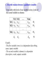
Tài liệu Slide bài giảng môn Lý thuyết xác suất thống kê bằng Tiếng Anh StatisticsLecture4B_HypothesisTest

Hypothesis tests for two independent
samples
•
Compare two proportions
•
Compare mean values of two populations
•
Compare two variances



Problem 3. Compare two mean values
1 2
( , , , )
n
X X X
1 2
( , , , )
m
Y Y Y
2
µ
Let be a sample of n independent
observations from a variable X with expectation and
variance
be a sample of m independent
observations from a variable Y with expectation and
variance
Problem: Compare two expectations and .
 Estimate and compare two mean values and .

1
µ
2
µ
2
2
σ
2
1
σ
YX
1
µ

The problem can be solved by using the following Theorem:
1 2
( , , , )
m
Y Y Y
2
Y
S
1 2
( , , , )
n
X X X
Theorem. Let and be two
samples of n independent observations selected correspondingly from
a variable X with sample mean and sample variance and
from a variable Y with sample mean and sample variance

(both variables are normal distributed). Then the (new) variable
has Student distribution with (n+m-2) degrees of freedom.
X
Y
2 2
. 2
. .( )
. .
X Y
n m n m
t X Y
n m
n S m S
+ −
= −
+
+
2
X
S

Hypothesis Tests
A. Two-tail Test: Hypothesis
H: Mean(X) = Mean(Y)
Alternative Hypothesis
K: Mean(X) differs from Mean(Y)
B. Right one-tail Test: Hypothesis
H: Mean(X) = Mean(Y)
Alternative Hypothesis K: Mean(X) > Mean(Y)
C. Left one-tail Test: Hypothesis

H: Mean(X) = Mean(Y)
Alternative Hypothesis K: Mean(X) < Mean(Y)

Steps of testing
Step 1. Estimate sample mean values Mean(X) , Mean(Y)
and sample variances Var(X) , Var(Y)
. 2
. .( ( ) ( ))
. ( ) . ( )
n m n m
t Mean X Mean Y
n m n Var X m Var Y
+ −
= −
+ +
Step 2. Calculating perform the quantity

Step 3 (Version A- Computer). Taking a variable
T(n+m-2) of Student distribution with (n + m - 2)
degrees of freedom calculate the probability
b = P { |T(n+m-2)| >= | t | }
(for 2-tails test); or
b = P { T(n+m-2) >= t }
(for right 1-tail test); or
b = P { T(n+m-2) =< t }
(for left 1-tail test, then t < 0 )

Step 4. Compare the probability b with a given ahead
significance level alpha (=5%, 1%, 0.5% or 0.1%):
+ If b >= alpha  accept Hypothesis H and conclude

Mean(X) = Mean(Y)
+ If b < alpha  reject Hypothesis H and confirm
Mean(X) kh¸c Mean(Y)
(for 2-tails test); or
Mean(X) > Mean(Y)
(for right 1-tail test); or
Mean(X) < Mean(Y)
(for left 1-tail test)

Version B. Using Student distribution table
Looking in Table of Student distribution find out
critical value T(n+m-2,alpha/2) of Student
distribution with n+m-2 degrees of freedom
( alpha is a given ahead significance level =5%,
1% or 0.5%)
Decide
- Reject Hypothesis H: = if
t > T(n+m-2,alpha/2)
- Accept Hypothesis H: = if
t =< T(n+m-2,alpha/2)

Version C. Using confidence intervals
When degree of freedom (sample size) is large,
Student distribution approximates Normal distribution.
Then we can use confidence intervals (with
significance level of 5%) for testing:
( ) 1.96* ( ) / ; ( ) 1.96* ( ) /Mean X Var X n Mean X Var X n
 
− +
 

Decide
Reject Hypothesis H: = if the two intervals disjoin
Accept Hypothesis H: = if the two intervals have
nonempty intersection
( ) 1.96* ( ) / ; ( ) 1.96* ( ) /Mean Y Var Y m Mean Y Var Y m
 
− +
 

SPSS

Test 4. Compare two independent samples -
Mann-Whitney non-parametric Test
Test 3 is powerful under assumption of Normal
distribution of variables X and Y , or sample
sizes n and m are large (>40). Without the above
assumption we must use “non-parametric“
methods

Mann-Whitney Test is a non-parametric test comparing
2 independent samples with Hypothesis
H: two variables X and Y have common distribution
(two samples have been selected from a homogeneous
population)
and Alternative Hypothesis
K: distributions of X and Y are different
(two sample have been selected from different
populations)

Non-parametric tests are based on comparing ranks of

values of concerned variables instead of comparing
directly the values of variables.
1 1
( ) if
p p p p
k k k k
h a p a a a
− +
= < <
1 2
, , ,
n
a a a
Definition. Given a sequence of
numbers. Let the sequence be reordered into increasing
sequence
Then rank h(.) of elements in the original sequence is
defined as the follows:
1 2

n
k k k
a a a≤ ≤ ≤
1 1 1
(2 )
( )
2
if
p
r r r p r s r s

k
k k k k k k
r s
h a
a a a a a a
− + + + +
+
=
< = = = = = <


Procedure of Testing
1
1
2
1
Determine the rank of each element in that sequence
and calculate the ranks sum of each sample:
(sum of ranks in the first sam= ( )
= (
ple)
(sum of ran s ) k i
n
i
i
n
j
j
R h X
R h Y

=
=
∑
∑
n the second sample)
Step 1:
1 2 1 2
( , , , ) ( , , , )Put together two sample and
into a common sequence of ( numbe) rs,
n m
X X X Y Y Y
n m+

1 1
2 2
1 2
Determine the rank statistics:




( 2)
.
2
( 2)
.
2
.
( , ) ;
2

. .( 1)
12
U
n n
U n m R
m m
U n m R
n m
U min U U U
n m n m
S
+
= + −
+
= + −
= =
+ −
=
Step 1 (continued):

1 2 1 2
LEMMA. Suppose ( , , , ) and ( , , , ) be independent
samples from two continous varables and . Suppose that hypothesis
H is true. Then variable has distribution converging very fast
n m
X X X Y Y Y
X Y
U
2
to the

Normal distribution ( , ) , therefore the distribtion of the variable

converges very fast to the standard Normal distribution (0,1).
U
U
N U S
U U
u
S
N
−
=
REMARK. In the above Lemma, to conclude that
distributions of U and u are close to normal distributions
it is enough to have the sample sizes greater than 8.

Steps of Hypothesis testing
Step1. Determine rank of each element in both
samples and the quantity u as presented above;
Step2. Taking a variable N(0,1) with standard
normal distribution (normal distribution with
expectancy 0 and variance 1) canculate the
probability
b = P { | N(0,1) | > | u | }

Step 3. Compare the probability b with a given ahead
significance level alpha :
* If b > alpha  accept hypothesis H and
consider two variables X , Y as those have the same
distribution, i.e. both samples were selected from a

common homogeneous population
* If b <= alpha  reject hypothesis H and
conclude X , Y are truly different, i.e. the two samples
were taken from two different sources

Remark
In the above, T – tests are used for comparing mean
values and are valid if sample size are large (> 40)
or the condition of Normal distribution are fulfilled
The non-parametric Mann-Whitney test is used to
compare two medians, is applicable even when there
is no assumption of Normal distribtion and sample
sizes are not very large. When the sample size are
large the non-parametric and T tests are equivalent

Test 7. Compare two variances
Variance represents precision of a measure or of an
estimation. The smaller variance corresponds the
more accurate measure. Therefore the evaluation of
measure’s accuracy can be done by comparing
variances. The comparison can be processed by
assess ratio of two variances.

Testing problem
1 2 1 2
2 2
1 1 2 2
Let ( , , , ) and ( , , , ) be samples taken from
two Normal variables ~ ( , ) and ~ ( , ) .
n m

X X X Y Y Y
X N Y N
µ σ µ σ
2 2
1 2
2 2
1 2
Hypothesis H:
Alternative hypothesis K:
σ σ
σ σ
=
≠

Steps of testing process
2 2
2
2 2
2
2
2
Estimate sample variances and perfom the ratio
= if
=
,
( 1)
if
( 1)
( 1)
(

Step 1.
1)
X Y
X
X Y
Y
Y
X
S S
S n
F S S
S m
S m
F
S n
or
−
>
−
−
−
2 2

Y X
S S>

1 2 1 2
LEMMA. Suppose ( , , , ) and ( , , , ) be
independent samples from two Normal distributed varables and .
Suppose that hypothesis H is true. Then the ratio is a variable

with Fisher-S
n m
X X X Y Y Y
X Y
F
nedecordistribution of and degree of freedom
(for the first case) or and degree of freedom (for the second case).
n m
m n

Fisher (F) distribution
Parameter of Fisher distribution is “degree of
freedom“
1 2
( , )
ν ν