Đề thi Olympiad Á Châu 2015 - Bài 1 môn vật lý
Bạn đang xem bản rút gọn của tài liệu. Xem và tải ngay bản đầy đủ của tài liệu tại đây (205.72 KB, 4 trang )
1 / 4
Question 1
The fractional quantum Hall effect (FQHE) was discovered by D. C. Tsui and H.
Stormer at Bell Labs in 1981. In the experiment electrons were confined in two
dimensions on the GaAs side by the interface potential of a GaAs/AlGaAs
heterojunction fabricated by A. C. Gossard (here we neglect the thickness of the
two-dimensional electron layer). A strong uniform magnetic field was applied
perpendicular to the two-dimensional electron system. As illustrated in Figure 1, when
a current was passing through the sample, the voltage
H
across the current path
exhibited an unexpected quantized plateau (corresponding to a Hall resistance
H
=
3/
2
) at sufficiently low temperatures. The appearance of the plateau would imply
the presence of fractionally charged quasiparticles in the system, which we analyze
below. For simplicity, we neglect the scattering of the electrons by random potential,
as well as the electron spin.
(a) In a classical model, two-dimensional electrons behave like charged billiard balls
on a table. In the GaAs/AlGaAs sample, however, the mass of the electrons is
reduced to an effective mass
due to their interaction with ions.
(i) (2 point) Write down the equation of motion of an electron in perpendicular
electric field
=
and magnetic field
= .
(ii) (1 point) Determine the velocity
s
of the electrons in the stationary case.
(iii) (1 point) Which direction is the velocity pointing at?
(b) (2 points) The Hall resistance is defined as
H
=
H
/. In the classical model,
find
H
as a function of the number of the electrons and the magnetic flux
= = , where is the area of the sample, and and the
effective width and length of the sample, respectively.
(c) (2 points) We know that electrons move in circular orbits in the magnetic field. In
the quantum mechanical picture, the impinging magnetic field could be
viewed as creating tiny whirlpools, so-called vortices, in the sea of
electrons—one whirlpool for each flux quantum / of the magnetic field,
where is the Planck's constant and the elementary charge of an electron.
For the case of
H
= 3/
2
, which was discovered by Tsui and Stormer, derive
the ratio of the number of the electrons to the number of the flux quanta
,
2 / 4
known as the filling factor .
Figure 1: (a) Sketch of the experimental setup for the observation of the FQHE. As indicated, a
current is passing through a two-dimensional electron system in the longitudinal direction with
an effective length . The Hall voltage
H
is measured in the transverse direction with an effective
width . In addition, a uniform magnetic field is applied perpendicular to the plane. The
direction of the current is given for illustrative purpose only, which may not be correct. (b) Hall
resistance
H
versus at four different temperatures (curves shifted for clarity) in the original
publication on the FQHE. The features at
H
= 3/
2
are due to the FQHE.
(d) (2 points) It turns out that binding an integer number of vortices ( > 1) with
each electron generates a bigger surrounding whirlpool, hence pushes away all
other electrons. Therefore, the system can considerably reduce its electrostatic
3 / 4
Coulomb energy at the corresponding filling factor. Determine the scaling
exponent of the amount of energy gain for each electron ()
.
(e) (2 points) As the magnetic field deviates from the exact filling = 1/ to a
higher field, more vortices (whirlpools in the electron sea) are being created.
They are not bound to electrons and behave like particles carrying effectively
positive charges, hence known as quasiholes, compared to the negatively charged
electrons. The amount of charge deficit in any of these quasiholes amounts to
exactly 1/ of an electronic charge. An analogous argument can be made for
magnetic fields slightly below and the creation of quasielectrons of negative
charge
= /. At the quantized Hall plateau of
H
= 3/
2
, calculate the
amount of change in that corresponds to the introduction of exactly one
fractionally charged quasihole. (When their density is low, the quasiparticles are
confined by the random potential generated by impurities and imperfections,
hence the Hall resistance remains quantized for a finite range of .)
(f) In Tsui et al. experiment,
the magnetic field corresponding to the center of the quantized Hall plateau
H
= 3/
2
,
1/3
= 15 Tesla,
the effective mass of an electron in GaAs,
= 0.067
,
the electron mass,
= 9.1 × 10
31
kg,
Coulomb's constant, = 9.0 × 10
9
N m
2
/C
2
,
the vacuum permittivity,
0
= 1/4 = 8.854 × 10
12
F/m,
the relative permittivity (the ratio of the permittivity of a substance to the vacuum
permittivity) of GaAs,
= 13,
the elementary charge, = 1.6 × 10
19
C,
Planck's constant, = 6.626 × 10
34
J s, and
Boltzmann's constant,
B
= 1.38 × 10
23
J/K.
In our analysis, we have neglected several factors, whose corresponding energy
scales, compared to () discussed in (d), are either too large to excite or too
small to be relevant.
(i) (1 point) Calculate the thermal energy
th
at temperature = 1.0 K.
(ii) (2 point) The electrons spatially confined in the whirlpools (or vortices) have
a large kinetic energy. Using the uncertainty relation, estimate the order of
magnitude of the kinetic energy. (This amount would also be the additional
energy penalty if we put two electrons in the same whirlpool, instead of in
two separate whirlpools, due to Pauli exclusion principle.)
(g) There are also a series of plateaus at
H
= /
2
, where = 1, 2, 3, … in Tsui et
al. experiment, as shown in Figure 1(b). These plateaus, known as the integer
quantum Hall effect (IQHE), were reported previously by K. von Klitzing in 1980.
Repeating (c)-(f) for the integer plateaus, one realizes that the novelty of the
FQHE lies critically in the existence of fractionally charged quasiparticles. R.
4 / 4
de-Picciotto et al. and L. Saminadayar et al. independently reported the
observation of fractional charges at the = 1/3 filling in 1997. In the
experiments, they measured the noise in the charge current across a narrow
constriction, the so-called quantum point contact (QPC). In a simple statistical
model, carriers with discrete charge
tunnel across the QPC and generate
charge current I
B
(on top of a trivial background). The number of the carriers
arriving at the electrode during a sufficiently small time interval obeys Poisson
probability distribution with parameter
P
(
=
)
=
e
!
where ! is the factorial of . You may need the following summation
e
=
!
k=0
(i) (2 point) Determine the charge current
B
, which measures total charge per
unit of time, in terms of and .
(ii) (2 points) Current noise is defined as the charge fluctuations per unit of time.
One can analyze the noise by measuring the mean square deviation of the
number of current-carrying charges. Determine the current noise
due to
the discreteness of the current-carrying charges in terms of and .
(iii) (1 point) Calculate the noise-to-current ratio
/
B
, which was verified by R.
de-Picciotto et al. and L. Saminadayar et al. in 1997. (One year later, Tsui
and Stormer shared the Nobel Prize in Physics with R. B. Laughlin, who
proposed an elegant ansatz for the ground state wave function at = 1/3.)