Proceedings VCM 2012 42 mô hình hóa và mô phỏng phương tiện ngầm vận hành từ xa

312 Hung Duc Nguyen, Sachith Malalagama and Dev Ranmuthugala


VCM2012
Modelling and Simulation of a Remotely Operated Vehicle
Mô hình hóa và mô phỏng phương tiện ngầm vận hành từ xa
Hung Duc Nguyen, Sachith Malalagama and Dev Ranmuthugala
University of Tasmania / Australian Maritime College
e-Mails:
Abstract
This paper presents modelling of a newly-built remotely operated vehicle utilising theoretical and CFD
simulation methods and the development of simulation programs to predict the behaviour of the ROV using
LabVIEW. In order to design and to implement precise control of a ROV during missions, mathematical
models with hydrodynamic coefficients are required. Hydrodynamic coefficients of the proposed mathematical
model are determined by analytical and CFD simulation methods supplemented by experimental work. A
computer simulation is developed to verify the coefficients and mathematical model of the ROV under various
manoeuvres.
Tóm tắt:
Bài báo trình bày mô hình hóa thiết bị ngầm vận hành từ xa mới đuợc thiết kế bằng hai phương pháp lý
thuyết và mô phỏng CFD và sự phát triển chương trình mô phỏng để ước ược động thái của thiết bị ngầm dùng
LabVIEW. Nhằm thiết kế và thực hiện điều khiển chỉnh xác một thiết bị ngầm vận hành từ xa trong khi làm
nhiệm vụ thì cần có mô hình toán có đầy đủ hệ số thủy động học. Các hệ số thủy động học của mô hình toán
được xác định bằng phương pháp giải tích và mô phỏng CFD có phụ trợ bằng thực nghịệm. Mô phỏng được
thực hiện nhằm kiểm chứng các tham số và mô hình toán của thiết bị ngầm vận hành từ xa theo các điều động
khác nhau.


Nomenclature
Symbol

Unit

Meaning

ν




T
u,v,w,p,q,r
ν
η




T
n,e,d, , ,
   
η
M


Mass matrix

D


Damping matrix

C


Coriolis matrix

G


Vector
of gravitational and
buoyancy forces and
moments
B

N

Buoyancy force

W

N

Weight

U


Vector of inputs

x

G
, y
G
, z
G

m

Coordinates of the centre of
gravity
l
i

(i=1,2,3)

Distance from each thruster
to centre of gravity
Abbreviation
CFD

Computational
F
luid
D
ynamics

DOF

Degree of
F

reedom

ROV

Remotely
O
perated
V
ehicle

AUV

Autonomous
U
nderwater
V
ehicle

HIL

Hardware
I
n the
L
oop

AMC

Australian Maritime College

UTAS

University of Tasmania


1. Introduction

When designing ROV/AUV platforms as in
[11][12] for educational and research work, the
physical and virtual/mathematical models play an
important role enabling the designer to understand
its dynamics and to develop its control system.
However the development of a specialist physical
prototype of a ROV or AUV with off the shelf
electronics is relatively expensive and in many
cases prohibitive within undergraduate
programmes. The work in this paper incorporates
the development of an inexpensive ROV using
easily accessible materials.
Although the vehicle in this paper is tethered, i.e.
an ROV generally depends on a human operator
for the guidance and control [22], it can also be
untethered with pre-programmed mission control
and both. The ROV described in this paper was
fabricated using PVC piping, submersible bilge
pump motors connected to model scale propellers,
fishing floats and accessories that are easily
obtainable from the local hardware shops.
The ROV was designed to carry out the following
tasks [17][ 18]:

Tuyển tập công trình Hội nghị Cơ điện tử toàn quốc lần thứ 6 313


Mã bài: 67
 observe and survey seabed conditions and
submersed objects and structures;
 observe marine farm facilities and equipment;
and
 perform basic underwater surveillance
operations.
The work further develops the mathematical
models, control algorithms and computer
simulation to predict the dynamic behaviour of the
ROV. Thus this paper describes the:
 newly-built low cost ROV;
 modelling of the ROV/AUV using theoretical
and CFD methods;
 calculation of the hydrodynamic coefficients of
the ROV;
 simulation of the ROV under various
manoeuvring scenarios;
 design and simulation of a trajectory tracking
control system to conduct underwater missions;
and
 conduct experimental work to determine the
hydrodynamic coefficients and validation of the
model.

2. Description of AMC ROV-IV
AMC-ROV-IV was made of PVC pipes and joints,

aluminium frames, and two fishing floats as shown
in Fig. 1. Three motors from submerged bilge
pumps connected to model scaled propellers were
used as thrusters for propulsion and vertical
motion. All materials used were easily accessible
from a household hardware or marine supplier [18].
The main particulars of the ROV are given in
Table 1. The ROV has been tested for watertight
integrity to a depth of about 5 metres in the AMC
Survival Centre Swimming Pool and the
Circulating Water Channel.


Fig. 1 AMC ROV-IV
Table 1 Main particulars of AMC ROV-IV
Length overall [mm] 480
Width of frame [mm] 290
Horizontal distance
between centres of the
two main thrusters [mm]
180
Overall width [mm] 400
Height without floats
[mm]
190
Height with floats [mm] 225
Weight in air [kg] 2.965
Volume [m
3
] 2.946 x 10

-3


The ROV is equipped with the following sensors
and actuators:
 actuators/thrusters: three bilge pump motors;
 three switch (relay) motor controllers;
 two forward lights; and
 instrumentation and control electronics.

3. Reference Frames and Equations
3.1 Reference Frames
In the design of control systems for underwater
vehicles, their kinematics and kinetics are
described using the reference frames given in Fig.
2, which includes the Earth-centred reference
frames (the Earth-centred Earth-fixed frame x
e
y
e
z
e

and the Earth-centred inertial frame x
i
y
i
z
i
), and the

geographic reference frames (the North-East-
Down coordinate system x
n
y
n
z
n
and the body-fixed
reference frame x
b
y
b
z
b
) [3][4].

Fig. 2 The ECEF frame x
e
y
e
z
e
is rotating with
angular rate with respect to an ECI frame x
i
y
i
z
i

fixed in space [3][4].

The two reference frames for the AMC ROV are
shown in Fig. 3. NED is the earth-fixed reference
frame and XYZ is the body-fixed reference frame.
314 Hung Duc Nguyen, Sachith Malalagama and Dev Ranmuthugala


VCM2012
The centre of gravity G is at the vertical central
thruster. The arrangement of the three thrusters for
position control is shown in Fig. 4. Two floats plus
a set of adjustable weights are used to adjust the
position of the centre of buoyancy and the
vehicle’s pitch.

Fig. 3 Reference frames for AMC ROV-IV

3.2 Kinematics
Referring to Fig. 3, the 6-DOF kinematic
equations in the NED (north-east-down) reference
frame in the vector form are [3][4],




η J η ν

(1)
where

 
 
 
n
b 3 3
3 3

 
 

 
 
 
R Θ 0
J η
0 T
Θ
(2)
with
3 3
S
 
η

and
3
ν

.

Fig. 4 Arrangement of thrsuters of AMC ROV-IV
(u
i
, i = 1 to 3, are the voltage inputs of thrusters)

The angle rotation matrix


n 3 3
b

R Θ

is defined
in terms of the principal rotations as [3][4],
x,
1 0 0
0 c s
0 s c


 
 
   
 
 
 
 
R ,
y,
c 0 s
0 1 0
s 0 c

 
 
 

 
 
  
 
R and
z,
c s 0
s c 0
0 0 1

  
 
 

  
 
 
 
R (3)
where s

=sin(

), c

= cos(

).using the zyx-
convention,


n
b z, y, x,
:
  
R
Θ R R R
(4)
or
 
n
b
c c s c c s s s s c c s
s c c c s s s c s s s c

s c s c c
             
 
 
              
 
 
     
 
R Θ
(5)
The inverse transformation satisfies,
   
1
n b T T T
b n x, y, z,

  
 R
Θ R Θ R R R
(6)
The Euler angle attitude transformation matrix is:
 
1 s t c t
0 c s
0 s /c c /c

   
 
 

   
 
 
   
 
T Θ


 
1
1 0 s
0 c c s
0 s c c


 
 
 
   
 
 
   
 
T Θ where
o
90
  
(7)
It should be noted that




T
Θ
is undefined for a
pitch angle of
o
90
  
and that




1 T
 
T
Θ T Θ
.

2.3 Kinetics
The 6-DOF kinetic equations in the body-fixed
reference frame in the vector form are therefore
[3],







0 wind wave
      Mν C ν ν D ν ν g η g τ τ τ

(8)
where
M = M
RB
+M
A
: system inertia matrix (including
added mass)


C
ν
=




RB A
C
ν C ν
: Coriolis-centripetal matrix
(including added mass)


D
ν
: damping matrix



g
η
: gravitational/buoyancy forces and moments
vector
0
g
: pre-trimming (ballast control) vector
τ
: control input vector
wind
τ
: wind-induced forces and moments vector
wave
τ
: wave-induced forces and moments vector

G

u
2

u
1

u
3

x

y

Tuyển tập công trình Hội nghị Cơ điện tử toàn quốc lần thứ 6 315


Mã bài: 67
3.1 Mathematical Model with Environmental
Disturbances
In order to improve performance of the control
systems for underwater vehicles it is necessary to
consider the effects of external disturbances on the
vehicle, which include wind, waves and currents.
According to Fossen [3], for control system design
it is common to assume the principle of
superposition when considering wind and wave
disturbances. In general, the environmental forces
and moments will be highly nonlinear and both
additive and multiplicative to the dynamic
equations of motion. An accurate description of
the environmental forces and moments is
important in vessel simulators and provides useful
information to the human operators.
With effects of external disturbances Equation (8)
is rewritten as [3][4],







 
RB RB A r A r r r r
0
   
   
M
ν C ν ν M ν C ν ν D ν ν
g η g τ w
 
(9)
where
wind wave
 w
τ τ
and
r c
 
ν ν ν
(where
6
c
ν

is the velocity of the ocean current
expressed in the NED). Further information on
modelling environmental disturbances can be
found in [2][3].
The model without external forces and moments
[3], [4] and [10] is









   M
ν C ν ν D ν ν g η B η u

(10)

3.2 Mathematical Models for ROV
In order to derive the differential equations
governing the kinematics and dynamics of the
vehicle of which inputs and outputs are shown Fig.
5, it is assumed that:
 the origin of the body-fixed reference frame is
at the centre of gravity where the vertical
thruster is located;
 the vehicle is symmetric about the longitudinal
axis x;
 the body has an equivalent block shape; and
 the vehicle is neutrally buoyant and the mass
distribution of the vehicle is homogeneous
throughout the vehicle.
Thus, the 6-DOF model in Equation (9) is applied
to the AMV ROV as follows [2][3][4][10].
Equations for kinematics:




η J η ν

(11)

Fig. 5 Input and output variables of the AMC
ROV/AUV-IV

Equations for kinetics:




   M
ν C ν ν D ν ν g Bu

(12)
where
x
y
z
 
 
 
 

 

 

 

 

 
 
η
;


J
η
as in equation (2);
u
v
w
p
q
r
 
 
 
 

 
 
 
 
 
 

ν
;

u
v
w
x p
y q
z r
m X 0 0 0 0 0
0 m Y 0 0 0 0
0 0 m Z 0 0 0
0 0 0 I K 0 0
0 0 0 0 I M 0
0 0 0 0 0 I N

 
 

 
 

 
 

 
 

 


 
 
M






w v
w u
v u
w v z r y q
w u z r x p
v u y q x p
0 mr mq 0 Z w Y v
mr 0 mp Z w 0 X u
mq mp 0 Y v X u 0
( )
0 Z w Y v 0 (I N )r (I M )q
Z w 0 X u (I N )r 0 (I K )p
Y v X u 0 (I M )q (I K )p 0
 
 
 
 
 
 
 


 
   
 
 
   
 
    
 
 
C ν
 
 
 
 
 
  
 
 

u
uu
v
vv
w
ww
p
pp
q
qq
r

r r
X X u 0 0 0 0 0
0 Y Y v 0 0 0 0
0 0 Z Z w 0 0 0
( )
0 0 0 K K p 0 0
0 0 0 0 M M q 0
0 0 0 0 0 K K r
  
 

 
 

 

 

 
 

 
 

 
D ν
B
B
0
0

0
( )
z Bcos sin
z Bsin
0
 
 
 
 

 
 
 
 

 
 
g η
;
1 2 3
3 3
k k 0
0 0 0
0 0 k
0 0 0
kl kl kl
kl kl 0
 
 
 

 

 
 
 

 
 
 
B
;
and
1
2
3
u
u
u
 
 

 
 
 
u .
The determination of all coefficients of (12) is
discussed in the following sections.

4. Parameter Identification
316 Hung Duc Nguyen, Sachith Malalagama and Dev Ranmuthugala

VCM2012
4.1 Theoretical Parameter Estimation
Translational added mass of the vehicle due to the
translational accelerations were determined by the
analytical method using the geometrical
parameters of the vehicle (see Table 1).
The added mass for each direction of translational
motion, i.e. surge, sway and heave were calculated
for each component and then added arithmetically
to obtain the added mass for the complete ROV for
the given direction.
Where the added masses for two dimensional
potential flows are not available, the projected area
of a particular component for the given direction
was obtained and using its principle dimensions
the added mass in the given direction was
calculated using the following formula [24][29].
2 2
i i
ii
i i
(a )(b )
4
M
3 (a b )




(13)
where M
ii
= translational added mass and a
i
, b
i
=
two principal dimensions of the projected area (b
i

> a
i
).
The values of added mass in three directions are
given in Table 2.

Table 2 Estimated added mass in three directions
Added mass Added mass [kg]
Surge 1.251
Sway 1.919
Heave 2.11

For estimation of added moments of inertia, it is
assumed that the added moment of inertia around
each axis of rotation is represented by half of the
moment of inertia around the particular axis as
given in Table 3.

Table 3 Estimated added moments of inertia

Axis of
rotation
Moment of
inertia (kgm
2
)
Added
moment of
inertia(kgm
2
)
X I
x
= 0.067
p
K

=0.0335
Y I
y
= 0.091
q
M

= 0.045
Z I
z
= 0.05
r
N


= 0.025

4.2 Experimental Parameter Estimation
The geometrical parameters measured are given in
Table 4 and the experimentally determined mass
and moments of inertia are given in Table 5.

Table 4 Geometrical parameters of the ROV
Vertical distance between port and
STBD thrusters to centre of gravity
(l
1
)
0
[mm]
Longitudinal distance between
vertical thrusters and centre of
gravity (l
2
)
0
[mm]
Horizontal distance between Port
and STBD thrusters to centre of
gravity (l
3
)
180
[mm]

Table 5 Mass and inertia properties
Parameter Value
Mass (m) 2.965 kg
Moment of inertia around
x- axis (I
x
)
0.067072131
kgm
2

Moment of inertia around
y-axis (I
y
)
0.091018248
kgm
2

Moment of inertia around
z- axis (I
z
)
0.050413326
kgm
2


To determine the damping coefficients a series of

experiments were carried out to measure the
damping forces acting on the ROV in different
orientations. These experiments were conducted in
the AMC Circulating Water Channel shown in Fig.
6.


Fig. 6 Schematic diagram of the CWC

In this project the forces acting on the umbilical
were not considered. Hence, the experiments were
carried out only on the ROV (vehicle) as follows:
 The ROV was detached from the umbilical.
 As the ROV is slightly positively buoyant,
ballast weights were attached to the ROV to
make it negatively buoyant.
 Loops were attached to the neutral axis of the
ROV as shown in Fig. 7.
 A load cell was calibrated with known weights.
Tuyển tập công trình Hội nghị Cơ điện tử toàn quốc lần thứ 6 317


Mã bài: 67
 The ROV was then attached to the load cell
from the loops.
 ROV was submerged in the circulating water
channel and the circulation of water was
initiated.
 The calculated drag forces from the
experiments are plotted together with the

corresponding drag forces obtained from
computational fluid dynamics simulations.
 The experimental results were non-
dimensionalised and then compared with the
CFD simulation results in order to validate the
obtained model.


Fig. 7 Attachment of loops to approximately to the
neutral axis
Fig. 8 shows the experiment being carried out for
the surge direction. Fig. 9 shows the comparison
of the total drag force obtained by the experiments
for the surge orientation to that obtained by CFD.
It can be seen from Fig. 9 that the experimental
results and the CFD simulation results are
sufficiently similar.

Fig. 8 Drag test in the surge orientation

Fig. 9 Drag force against flow velocity for surge
orientation

Fig. 10 and Fig. 11 show drag test and the graph
of drag force vs the flow velocity for sway
orientation.

Fig. 10 Drag test in the sway orientation

Fig. 11 Drag force against flow velocity for sway
orientation
Fig. 12 and Fig. 13 show the drag force in the
heave orientation and the respective graph of the
drag force vs the flow velocity.
318 Hung Duc Nguyen, Sachith Malalagama and Dev Ranmuthugala


VCM2012

Fig. 12 Drag test in the heave orientation

Fig. 13 Drag force against flow velocity for heave
orientation

4.3 Thruster Coefficient Identification
The thruster coefficient matrix and the thruster
input matrix were determined based on the
assumption that the characteristics of all three
thruster motors used in the ROV were identical.
The experiment setup is shown in Fig. 14 and Fig.
15.


Fig. 14 Experiment setup for thruster coefficient
determination

Fig. 15 Experiment setup in the laboratory

Fig. 16 shows the graph of the thruster force vs the

supply voltage. It is seen that from the graph no
thrust is generated when the supply voltage is less
than 2 V. Hence, the value of thrust force
coefficient, k was found as,
k = 0.373 N/V.

Fig 16 Thruster force vs supply voltage

4.4 CFD Method
Simulations of the ROV using a CFD model were
used to determine the linear and quadratic
damping derivatives. The results obtained from the
CFD analysis were validated against the
Tuyển tập công trình Hội nghị Cơ điện tử toàn quốc lần thứ 6 319


Mã bài: 67
experimental data. The CFD was carried out using
the commercial software ANSYS-CFX.

4.4.1 Geometry Creation
The 3D model used for the CFD was developed
using the AutoCAD and then imported into
ANSYS® Design Modeller in IGES 144 format.
In Design Modeller the fluid domain required for
the simulation was created. The complete
geometry is shown in Fig. 17 and Fig. 18.


Fig. 17 Flow domain plan front view

Fig. 18 Flow domain plan side view

4.4.2 Mesh Generation
Meshing is the discretization of the fluid domain
volume into adjoining finite volumes. Mesh
quality and distribution are critical to obtain
accurate results from a CFD simulation.
The entire fluid domain mesh was created with the
automatic method control, as shown in Fig. 19.
The mesh independence study was carried out by
changing the curvature normal angle from 18
o
to
4.5
o
. The rest of the settings were kept constant.

4.4.3 Mesh Independence
A mesh independence study was done in order to
establish the results obtained from the CFD
simulations independent of the number of
elements in the mesh. Fig. 19 shows overall mesh
of the ROV. The number of elements of the mess
was changed by varying changing the curvature
normal angle as shown in Table 6.


Fig. 19 Overall mesh of the ROV

Table 6 Changed setting for mesh independence
study
(*) Quadratic damping derivative in the surge
direction

The quadratic damping derivatives obtained with
different mesh sizes for the surge direction are
plotted in Fig. 20 [22]. By considering the
accuracy compared to the experimental results as
in Section 4.2 and the time available time for
simulations it could be concluded that the mesh
generated with a 9
o
curvature normal angle is the
most suitable to carry out the rest of simulations.
Curvature
normal
angle
Number of
Elements
u u
X
(*)
18
o
2150311 15.58
13.5
o
2875855 13.31

9
o
4590472 10.88
6.5
o
8171510 10.07
4.5
o
9164514 10.07
320 Hung Duc Nguyen, Sachith Malalagama and Dev Ranmuthugala


VCM2012


Fig. 20 Quadratic damping coefficients
u u
X

against the number of elements

4.4.4 Physics and Fluid Properties
When running the CFD simulations it was
necessary to set physical and fluid properties used
for translational and rotational motions. These
properties are summarised in Tables 7 and 8.

Table 7 Flow physics used for the CFD simulation
(translational)

Table 8 Flow physics used for the CFD simulation
(rotational)




4.4.5 Boundary Conditions

Boundary conditions for translational motion and
rotational motion are shown in Tables 9 and 10.

Table 9 Boundary conditions (translational)

Table 10 Boundary conditions (rotational motion)


4.4.6 CFD Simulation Results
This section presents some of CFD simulation
results for translational motion, rotational motion
and hydrodynamic lift.

4.4.6.1 Translational Motion
Translational motion includes surge, sway and
heave. Table 11 and Fig. 21 through to 23 show
main results from the CFD simulation by which
coefficients were determined.

Table 11 CFD simulation results (translational)
Tuyển tập công trình Hội nghị Cơ điện tử toàn quốc lần thứ 6 321

Mã bài: 67



Fig. 21 Drag force vs velocity (surge)


Fig. 22 Drag force vs velocity (sway)

Fig. 23 Friction drag force vs velocity (heave)




4.4.6.2 Rotational Motion
Rotational motion of the ROV includes roll, pitch
and yaw. The CFD simulation results are
summarised in Table 12 and Fig. 23 through to 25.

Table 12 CFD simulation results for rotational
motion



Fig. 23 Torque vs angular velocity (roll)


Fig. 24 Torque vs angular velocity (pitch)
322 Hung Duc Nguyen, Sachith Malalagama and Dev Ranmuthugala

VCM2012

Fig. 25 Torque vs angular velocity (yaw)

4.3.3 Hydrodynamic Lift
Consistent with the observations made during the
testing of the vehicle, the CFD results indicated
the presence of hydrodynamic lift force during the
surge motion as shown in Fig. 26.

Fig. 26 Lift force vs velocity (surge)

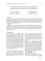
5. Simulation Study – Control Design
The automatic control system for the ROV as a
whole is illustrated in Fig. 27 showing the signal
flow of guidance, navigation and control systems.
Guidance system: to receive prior information,
predefined inputs, waypoints and generate desired
trajectory including desired speed, depth (heave),
yaw and position. A joystick may be used to
generate reference signals [3][4][7][23].

Fig. 27 Guidance, navigation and control systems

Navigation system: equipped with GNSS/INS
receivers and other sensors to provide
measurement of speed, depth, yaw and position
[3][4][7].

Control system: to detect error by comparing
actual speed, depth, heading angle and position
with desired values and calculating control signals
to be sent to the controller allocation devices
(actuators) [3][4][7].

The computer simulation using the above
mathematical model was developed using National
Instruments LabVIEW 2010. This allowed the
verification of the developed mathematical model
and the estimated hydrodynamic coefficients. A
number of simulated manoeuvres were carried for
this purpose.
As the first step to realize a hardware-in-the-loop
system, computer simulation programs were
developed using the mathematical model described
in Equations (10) and (11). A number of tests were
carried out for the simulation programmes
including:
 open-loop system manoeuvres;
 closed-loop system tests
 course control (course keeping and changing);
 speed, depth (heave) and pitch control;
 roll, surge and sway; and
 trajectory tracking control.

In the simulation programs for closed-loop control
systems (including depth and course keeping, pitch
and roll control, and position/trajectory tracking
control) the conventional PID control law was

used due to its simplicity, i.e.:
   


P I D
de t
u K e t K e t dt K
dt
  

(13)

5.1 Open-loop System Manoeuvres
Simulation for open-loop system manoeuvres was
done using equations (10) and (11) with estimated
parameters to investigate the ROV’s
characteristics without any control. The ROV’s
thrusters are controlled by three relay based motor
drives. The simulated manoeuvres presented here
include driving, course changing, course keeping,
and circular diving. More open-loop system
manoeuvres are currently being carried out, which
includes horizontal zigzag, horizontal turning
circle and depth zigzag tests.

Tuyển tập công trình Hội nghị Cơ điện tử toàn quốc lần thứ 6 323


Mã bài: 67
5.1.1 Manoeuvre 1: Diving, Course Changing

and Course Keeping
This basic manoeuvre enables the investigation
into the vehicle’s manoeuvrability. The vehicle
dives from the surface to a depth then turns to the
right at an angle, and travels in a straight line. The
simulated results are shown in Fig. 28 and Fig. 29.

5.1.2 Manoeuvre 2: Circular Diving
The circular diving manoeuvre simulation was
carried out to test the manoeuvring characteristic
(turning ability) of the ROV. Fig. 30 and Fig. 31
show simulated results for the circular diving
manoeuvre. It is seen from Fig. 30 and Fig. 31 that
the ROV has a good turning ability.














Fig. 28 Trajectory of diving, turning and going
straight

0 20 40 60 80
0
0.2
0.4
Time (s)
Surge Rate (m/s)
0 20 40 60 80
-1
0
1
Time (s)
Sway Rate (m /s)
0 20 40 60 80
0
0.1
0.2
Time (s)
Heave Rate (m /s)
0 20 40 60 80
-1
0
1
Time (s)
Roll Rate (Rad/s)
0 20 40 60 80
-1
0
1
Time (s)
Pitch Rate (Rad/s )

0 20 40 60 80
-1
-0.5
0
Time (s)
Yaw Rate (Rad/s )

Fig. 29 Linear and angular velocities

Fig. 30 Trajectory of circular diving manoeuvre

Fig 31 Linear and angular velocities for
Manoeuvre 2
5.2 Closed-Loop Control Manoeuvres
A ROV/AUV often does various underwater
missions that are based on predefined trajectories,
for examples, water sampling, survey of
submerged pipelines and cables, or hydrographical
surveys. As the first step to realise a trajectory
tracking control system for a ROV close loop
control manoeuvring simulations of the ROV were
carried out.
In the tracking control algorithm, the way-points
tracking Light Of Sight (LOS) method was applied.
A set of waypoints (x
k
,y
k
,z
k

, k = 1, 2, 3, …, N)
were the inputs. A desired trajectory including
desired course (
d

), speed (u
d
) and position
(x
d
,y
d
,z
d
) was generated. The desired course was
found by [4][5][7][9],
 


 
k
1
d
k
y y t
k tan
x y t

 


 
 
 

 
(14)
The new course, depth and speed was selected by
the circle of acceptance method as follows
[4][5][7][9],
     
2 2 2
2
k k k 0
x x t y y t z z t R
     
     
     
(15)
where (x,y,z) is the current position, R
0
is often
chosen as two times of the vehicle length (2L)
324 Hung Duc Nguyen, Sachith Malalagama and Dev Ranmuthugala


VCM2012
[4][5]. A desired trajectory is generated based on a
simplified mathematical model for the ROV.

Fig. 32 shows simulated results of tracking control

for a desired 3D trajectory of which the waypoints
are defined as X
wp
= [0 10 10 0 0 0 0 -10 -10 0 0];
Y
wp
= [0 0 10 10 0 0 -10 -10 0 0 0]; and Z
wp
=
[0.08 0.08 0.08 0.08 -10 -10 -10 -10 –10 0.08]. It
can be seen from Fig. 32 that the ROV could well
be controlled tracking a pre-defined 3D trajectory.
Fig. 32 shows time history of rates.


Fig. 32 Trajectory for underwater mission

From above figures it can be seen that the
overshoots for system responses are very small or
zero because the control gains were selected using
simulators.

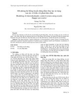
6. Electronics for Follow-up Experiments

In order to carryout various mission activities a
selection of instrumentation and control
electronics were installed onboard the ROV. Fig.
33 shows an arrangement of sensors, actuators and
target microcontroller (a cost-effective Arduino
board or Arduipilot board including

microcontroller and IMU/GPS module) and their
connection to a host PC with appropriate software.


Fig 33 Time history of rates



Fig. 34 Arrangement of sensors, actuators and
connection of the target microcontroller to the
host PC

Currently switch/relay motor drives have been
used to manoeuvre the ROV. In order to design
and implement an automatic control system for the
ROV, cost-effective electronic devices were
selected. It is planned to install an inexpensive
Arduino target microcontroller board and
electronics on the ROV in place of the
switch/relay motor drives. The estimated costs for
electronics are shown in Table 12 & Fig. 36.

The target computer (microcontroller) is connected
to the onshore host computer via an Ethernet or
USB cable or wireless (Xbee or RF). The host PC
is installed with control programmes developed
using software such as Arduino software (open
source), MATLAB / Simulink software or
LabVIEW.

Table 12 Estimated costs for electronics
Item Cost (AUD)
Arduino and
IMU/GPS boards
260
Tuyển tập công trình Hội nghị Cơ điện tử toàn quốc lần thứ 6 325


Mã bài: 67
Motor drives (3) 50
Electronics
components and
accessories
50
Wireless 80
Total 440

Fig 35 Target and host computers and software


Fig 36 Hardware including 1: motor drive (4
motors), 2. Breadboard, 3. Arduino Mega 2560, 4.
IMU and 5. GPS

7. Conclusions

The paper has described the:
 development of an inexpensive ROV using
easily accessible materials;
 reference frames for description of ROV

kinematics and kinetics;
 development of a mathematical model (6DOF)
using theoretical and CFD simulation methods;
 development of simulation programs and
design of experiments for various operational
scenarios; including: open-loop manoeuvres
and closed-loop control manoeuvres with PID
control law; and
 computer simulation results showing the
feasibility of the control algorithms for various
manoeuvres of ROVs.

Future work in this project will include:
 installation of electronic controls;
 development of high-performance control
programs using advanced or intelligent control
algorithms with LabVIEW or
MATLAB/Similnik or Arduino software;
 experimental work in the CWC, Survival Pool
or Model Test Basin;
 analyse of data from the experiments to verify
the mathematical models and the CFD
coefficients;
 experimental system identification methods and
experimental data for estimation of
hydrodynamic coefficients; and
 development of 3D trajectory tracking control
systems for complicated underwater missions.

References

[1] Roberts, G.N. and Sutton, R (Editors). Advances
in Unmanned Marine Vehicles. The Institute of
Electrical Engineers, 2006.
[2] Fossen, T.I Nonlinear Modelling and Control of
Underwater Vehicles, PhD Thesis. Norwegian
Institute of Technology, 1991.
[3] Fossen, T.I Handbook of Marine Craft
Hydrodynamics and Motion Control. John Wiley
and Sons Inc. 2011.
[4] Fossen, T.I Marine Control Systems –
Guidance, Navigation and Control of Ships, Rigs
and Underwater Vehicles. Marine Cybernetics,
Trondheim, Norway, 2002.
[5] Fossen, T.I Guidance and Control of Ocean
Vehicles. John Wiley and Sons, 1994.
[6] Wadoo, S.A. and Kachoroo, P Autonomous
Underwater Vehicles: Modeling, Control Design,
and Simulation. CRC Press, 2011.
[7] Nguyen, H.D Multitask Manoeuvring Systems
Using Recursive Optimal Control Algorithms.
Proceedings of HUT-ICCE 2008, pp. 54-59 Hoi
An, Vietnam, 2008.
[8] Nguyen, H.D Recursive Identification of Ship
Manoeuvring Dynamics and Hydrodynamics.
Proceedings of EMAC 2007 (ANZIAM), pp. 681-
697, 2008.
[9] Nguyen, H.D Recursive Optimal Manoeuvring
Systems for Maritime Search and Rescue
Mission, Proceedings of OCEANS'04
MTS/IEEE/TECHNO-OCEAN'04 (OTO’04), pp.

911-918, Kobe, Japan, 2004.
1

2

3

4

5

326 Hung Duc Nguyen, Sachith Malalagama and Dev Ranmuthugala


VCM2012
[10] Nguyen, HD and Pienaar, R and Ranmuthugala,
D and West, W, ‘Modeling, Simulation and
Control of Underwater Vehicles’, Proceedings of
The 1st Vietnam Conference on Control and
Automation, 25-26 November 2011, Hanoi,
Vietnam, pp. 150-159, 2011.
[11] West, W.J. Remotely Operated Underwater
Vehicle, BE Thesis. Australian Maritime College,
UTAS, Launceston, 2009.
[12] Gaskin, C.R Design and Development of
ROV/AUV, BE Thesis. Australian Maritime
College, UTAS, Launceston, 2000.
[13] Antonelli, G Underwater Robots – Motion and
Force Control of Vehicle-Manipulated Systems,
2

nd
Edition. Springer, 2006.
[15] Burcher, R. and L. Rydill Concepts in
Submarine Design. Cambridge University Press.
[16] Christ, R.D. and R.L. Wernli Sr (2007). The
ROV Manual – A User Guide for Observation
Class Remotely Operated Vehicles. Butter-
Heinemann (Elsevier). Oxford, 1994.
[17] Pienaar, R Simulation and Modelling of ROVs
and AUVs. BE Thesis. Australian Maritime
College, Launceston, 2011.
[18] Malalagama, S. Modelling and Simulation of a
Remotely Operated Vehicle, BE Thesis.
Australian Maritime College, University of
Tasmania, Launceston. 2012.
[19] Blohm, H. & Jensen, V. Build Your Own
Underwater Robot and Other Wet Projects,
Vancouver, Westcoast Words, 1997.
20] Brennen, C. E. A Review of Added Mass and
Fluid Inertial Forces. California: Naval Civil
Engineering Laborotary, 1982.
[21] Eng, Y. H., Lau, W. S., Low, E., Seet, G. G. L.
& Chin, C. S. Estimation of the Hydrodynamics
Coefficients of an ROV using Free Decay
Pendulum Motion. Engineering Letters, 2008.
[22] Fossen, T. I. Non Linear Modelling and Control
of Underwater Vehicles. Trondheim: Norwegian
Institute of Technology, 1987.
[23] Global Marine Oil Pollution Information
Gateway n.a. Global Marine Oil Pollution

Information Gateway - Oil - exploration and
extraction. .
[24] Heron, A., Woods, A. & Anderson, B.
Determination of Manoeuvring Coefficients for
the Triton ROV in the Circulating Water Channel.
Australian Maritime College, 2000.

Biography

Dr. Hung Nguyen is a
lecturer in Marine Control
Engineering at National
Centre for Maritime
Engineering and
Hydrodynamics, Australian
Maritime College, Australia.
He obtained his BE degree in
Nautical Science at Vietnam
Maritime University in 1991,
then he worked as a lecturer there until 1995. He
completed the MSc in Marine Systems
Engineering in 1998 at Tokyo University of
Marine Science and Technology and then the PhD
degree in Marine Control Engineering at the same
university in 2001. During April 2001 to July 2002
he worked as a research and development engineer
at Fieldtech Co. Ltd., a civil engineering related
nuclear instrument manufacturing company, in
Japan. He moved to the Australian Maritime
College, Australia in August 2002. His research

interests include guidance, navigation and control
of marine vehicles, self-tuning and optimal control,
recursive system identification, real-time control
and hardware-in-the-loop simulation of marine
vehicles and dynamics of marine vehicles.
Mr. Sachith Malalagama is a
final year Marine and
Offshore Engineering
student. Prior to his studies
at AMC he served as a
marine engineer and joined
AMC to further his
knowledge in maritime
engineering. Due to his
interest in underwater vehicles he undertook the
final year thesis “Modelling and Simulation of a
Remotely Operated Vehicle” which was carried
out under the guidance of Dr. Dev Ranmuthugala
and Dr. Hung Nguyen. Upon graduation he will be
employed as a mechanical and electrical design
engineer in the mining industry.

Dr Dev Ranmuthugala is the
Acting Director, National
Centre for Ports and
Shipping and Associate
Professor in Maritime
Engineering at the Australian
Maritime College,
University of Tasmania. He

has also served as Associate
Tuyển tập công trình Hội nghị Cơ điện tử toàn quốc lần thứ 6 327


Mã bài: 67
Dean, Teaching & Learning and as Head of
Department in Maritime Engineering and Vessel
Operations over the past 15 years. Prior to joining
AMC, he worked as a marine engineer and in the
design and sales of piping systems. His research
includes: experimental and computational fluid
dynamics to investigate the hydrodynamic
characteristics of underwater vehicles, behaviour
of submarines operating near the free surface,
stability of surfaced submarines, towed underwater
vehicle systems, and maritime engineering
education.

Appendix 1 Estimated Coefficients
Table A1.1 Estimated coefficients for (11) and
(12)
Coef. Value Coef
.
Value
L 480 mm
Widt
h
290 mm
m 2.965 kg I
x

0.067 kgm
2

I
y
0.091 kgm
2
I
z
0.05 kgm
2

B 29.08 m l
1
0
l
2
0 l
3
0.18 m
x
b
0 y
b
0
z
b
0 k 0.373 Nm/V
u
X



-1.251 kg
u u
X

-11.25 kgm
-1

v
Y


-1.919 kg
v v
Y

-16.22 kgm
-1

w
Z


-2.11 kg
w w
Z

-18.8 kgm
-1

p
K


-0.0335 kgm
2

p p
K

-0.07 kgm
q
M


-0.045 kgm
2

q q
M

-0.17 kgm
r
N


-0.025 kgm
2

r r
N

-0.11 kgm
u
X

-0.59 kgs
-1

p
K

-0.02 kgms
-1

v
Y

-0.66 kgs
-1

q
M

-0.06 kgms
-1

w
Z

-0.65 kgs
-1

r
N

-0.04 kgms
-1





Appendix 2 Snapshots of Simulation Program for Trajectory Tracking Control System

Fig. A2.1 Front Panel window of the simulation program

328 Hung Duc Nguyen, Sachith Malalagama and Dev Ranmuthugala


VCM2012

Fig. A2.2 Block diagram window (mathematical model) of the simulation program