Hidden markov model based methods in condition monitoring of machinery systems
Bạn đang xem bản rút gọn của tài liệu. Xem và tải ngay bản đầy đủ của tài liệu tại đây (3.44 MB, 166 trang )
Hidden Markov Model-Based Methods in
Condition Monitoring of Machinery Systems
BY
Omid Geramifard
B. Sc., Isfahan University of Technology
A THESIS SUBMITTED
FOR THE DEGREE OF DOCTOR OF PHILOSOPHY
DEPARTMENT OF ELECTRICAL AND COMPUTER ENGINEERING
NATIONAL UNIVERSITY OF SINGAPORE
2013
To my dear parents,
Vaji & Hadi,
for their everlasting love and support.
To my lovely wife,
Maryam,
whose presence lights me up and lifts up my spirit.
ii
Declaration
I hereby declare that the thesis is my original work and it is written by me in its
entirety. I have duly acknowledged all the sources of information which has been used
in this thesis.
This thesis has also not been submitted for any degree in any other university previously.
iii
Acknowledgment
First and foremost, I would like to express my deepest appreciation to my supervisor,
Professor Jian-Xin Xu for his invaluable guidance, patience and support in all aspects
of this research. The enthusiasm he has for research, was greatly motivational for me
during my Ph.D. pursuit. I am also grateful for the excellent example he has personified
as a mentor and professor.
I would sincerely thank my oral Qualification Examination committee members,
A/Professor Loh Ai Poh, A/Professor Geok Soon Hong and A/Professor Xiang Cheng,
for their kindness to review my report and give encouraging feedback.
I would also like to express my gratitude to Dr. Junhong Zhou, Dr. Xiang Li and
Dr. Oon Peen Gan from Singapore Institute of Manufacturing Technology (SIMTech),
who contributed immensely to this research by providing the experimental data and their
insightful advices.
I am truly thankful of all my friends and labmates for their companionship and
support throughout my Ph.D. journey; especially Deng Xin, Sidath R. Liyanage, Ren
Qinyuan, Zhaoqin Guo, Niu Xuelei, Deqing Huang, Yang Yue, Ramesh Bharath, Ehsan
Keikha, and Yohanes Daud. Also, I am very thankful to lab officers at Control and Sim-
ulation lab, Zhang Hengwei and Aruchunan Sarasupathi as well as all the staff members
at Department of Electrical and Computer Engineering and National University of Sin-
gapore for their kind support.
I would also like to specially thank my beloved wife Maryam Azh, my wonderful
parents Vajiheh and Hadi, and my siblings Ordin, Golnar and Negar for their eternal
love, support and encouragement; and my parents in-law, Parvin and Bahram for their
understanding and support.
iv
i
Lastly, I gratefully acknowledge the funding sources that made my Ph.D. work possi-
ble. My work has been supported by Singapore International Graduate Award (SINGA),
funded by Singapore Agency of Science, Technology and Research (A*STAR).
Contents
Summary vi
Nomenclature viii
List of Figures xii
List of Tables xv
1 Introduction 1
1.1 Background and Motivation of Research . . . . . . . . . . . . . . . . . 2
1.1.1 Tool Wear Monitoring . . . . . . . . . . . . . . . . . . . . . . 5
1.1.2 Fault Detection and Diagnosis in Rotary Electric Motors . . . . 7
1.1.3 Necessity of Temporal Models for Diagnostics and Prognostics 8
1.1.4 Hidden Markov Model . . . . . . . . . . . . . . . . . . . . . . 10
1.2 Objectives and Scope of Research . . . . . . . . . . . . . . . . . . . . 16
1.3 Contribution and Outline of Thesis . . . . . . . . . . . . . . . . . . . . 17
2 Physically Segmented Hidden Markov Model with Continuous Output 20
2.1 Introduction . . . . . . . . . . . . . . . . . . . . . . . . . . . . . . . . 20
2.2 Physically Segmented Hidden Markov Model with Continuous Output . 21
2.2.1 Discretization & Formulation . . . . . . . . . . . . . . . . . . 22
2.2.2 Parameter Estimation . . . . . . . . . . . . . . . . . . . . . . . 24
2.2.3 Forward-Backward Variables in PSHMCO . . . . . . . . . . . 27
2.2.4 State Estimation . . . . . . . . . . . . . . . . . . . . . . . . . 28
2.3 Diagnostics & Prognostics . . . . . . . . . . . . . . . . . . . . . . . . 29
ii
Contents iii
2.4 Experimental Data & Feature Selection . . . . . . . . . . . . . . . . . 31
2.5 Diagnostics & Prognostics Results . . . . . . . . . . . . . . . . . . . . 35
2.5.1 Determination of Hyper-parameters . . . . . . . . . . . . . . . 36
2.5.2 Diagnostic Results . . . . . . . . . . . . . . . . . . . . . . . . 37
2.5.3 Prognostic Results . . . . . . . . . . . . . . . . . . . . . . . . 41
2.6 Summary . . . . . . . . . . . . . . . . . . . . . . . . . . . . . . . . . 42
3 Hidden Semi-Markov Model-based Approach 44
3.1 Introduction . . . . . . . . . . . . . . . . . . . . . . . . . . . . . . . . 44
3.2 Hidden Semi-Markov Model-Based Approach . . . . . . . . . . . . . . 45
3.2.1 HMM Fixed Duration Distribution . . . . . . . . . . . . . . . . 45
3.2.2 Formulation and Parameter Estimation . . . . . . . . . . . . . . 46
3.2.3 Forward-Backward variables in PSHsMCO . . . . . . . . . . . 51
3.2.4 State Estimation . . . . . . . . . . . . . . . . . . . . . . . . . 53
3.3 Diagnostics & Prognostics . . . . . . . . . . . . . . . . . . . . . . . . 54
3.4 Diagnostics and Prognostics Results . . . . . . . . . . . . . . . . . . . 56
3.4.1 Cross-Validation Results . . . . . . . . . . . . . . . . . . . . . 56
3.4.2 Diagnostics Results . . . . . . . . . . . . . . . . . . . . . . . . 57
3.4.3 Prognostics Results . . . . . . . . . . . . . . . . . . . . . . . . 58
3.5 Asymmetric Loss Function . . . . . . . . . . . . . . . . . . . . . . . . 59
3.5.1 Asymmetric Cross-Validation . . . . . . . . . . . . . . . . . . 64
3.5.2 Asymmetric Diagnostics . . . . . . . . . . . . . . . . . . . . . 64
3.6 Summary . . . . . . . . . . . . . . . . . . . . . . . . . . . . . . . . . 65
4 Multi-Modal Hidden Markov Model-Based Approach 67
4.1 Introduction . . . . . . . . . . . . . . . . . . . . . . . . . . . . . . . . 67
4.2 Windowed Single HMM-based Approach . . . . . . . . . . . . . . . . 68
4.3 Multi Modal HMM-Based Approach . . . . . . . . . . . . . . . . . . . 69
4.3.1 Most Probable Health States . . . . . . . . . . . . . . . . . . . 70
4.3.2 Weighting Schemes . . . . . . . . . . . . . . . . . . . . . . . . 72
4.3.3 Switching Strategy . . . . . . . . . . . . . . . . . . . . . . . . 76
Contents iv
4.3.4 Windowing Algorithm for m
2
HMMs . . . . . . . . . . . . . . 78
4.4 Preliminary Experimental Results . . . . . . . . . . . . . . . . . . . . 78
4.4.1 Experimental Data and Features . . . . . . . . . . . . . . . . . 79
4.4.2 Preliminary Results . . . . . . . . . . . . . . . . . . . . . . . . 79
4.5 Further Investigations . . . . . . . . . . . . . . . . . . . . . . . . . . . 82
4.5.1 Switching Strategy: Hard Vs. Soft . . . . . . . . . . . . . . . . 84
4.5.2 Overall Performance Comparison . . . . . . . . . . . . . . . . 85
4.5.3 Full Vs. Windowed Observations . . . . . . . . . . . . . . . . 85
4.5.4 Reference Length Sensitivity Analysis . . . . . . . . . . . . . . 87
4.6 Summary . . . . . . . . . . . . . . . . . . . . . . . . . . . . . . . . . 90
5 Hidden Markov Model-Based Fault Detection and Diagnosis 91
5.1 Introduction . . . . . . . . . . . . . . . . . . . . . . . . . . . . . . . . 91
5.2 Rotary Machine Fault Mechanics . . . . . . . . . . . . . . . . . . . . . 93
5.3 Signature Squeezing & Stretching . . . . . . . . . . . . . . . . . . . . 95
5.3.1 Squeezing in Time . . . . . . . . . . . . . . . . . . . . . . . . 96
5.3.2 Stretching in Amplitude . . . . . . . . . . . . . . . . . . . . . 97
5.4 HMM-based Fault Diagnosis . . . . . . . . . . . . . . . . . . . . . . . 97
5.4.1 Conventional HMM-Based Classification . . . . . . . . . . . . 98
5.4.2 HMM-based Semi-Nonparametric Approach . . . . . . . . . . 100
5.5 Preliminary Experimental results . . . . . . . . . . . . . . . . . . . . . 105
5.5.1 Classification Accuracy . . . . . . . . . . . . . . . . . . . . . 106
5.5.2 Cost Analysis . . . . . . . . . . . . . . . . . . . . . . . . . . . 107
5.6 Further Investigations and Sensitivity Analysis . . . . . . . . . . . . . . 108
5.6.1 Overall Performance . . . . . . . . . . . . . . . . . . . . . . . 109
5.6.2 Hyper-parameter Sensitivity . . . . . . . . . . . . . . . . . . . 111
5.6.3 Signature Length Sensitivity . . . . . . . . . . . . . . . . . . . 112
5.7 Summary . . . . . . . . . . . . . . . . . . . . . . . . . . . . . . . . . 113
6 Conclusion and Future Work 115
6.1 Contributions . . . . . . . . . . . . . . . . . . . . . . . . . . . . . . . 115
Contents v
6.1.1 PSHMCO . . . . . . . . . . . . . . . . . . . . . . . . . . . . . 115
6.1.2 HSMM-based Approach . . . . . . . . . . . . . . . . . . . . . 116
6.1.3 Multi-modal HMM-Based Approach . . . . . . . . . . . . . . 117
6.1.4 Semi-Nonparametric HMM-based Classification . . . . . . . . 118
6.2 Future Work . . . . . . . . . . . . . . . . . . . . . . . . . . . . . . . . 118
Appendices
A Tool Wear in CNC-milling machine Dataset and Experimental Setup 123
A.1 Introduction . . . . . . . . . . . . . . . . . . . . . . . . . . . . . . . . 123
A.2 Dataset & Features . . . . . . . . . . . . . . . . . . . . . . . . . . . . 123
A.2.1 Statistical Features . . . . . . . . . . . . . . . . . . . . . . . . 124
A.2.2 Wavelet Features . . . . . . . . . . . . . . . . . . . . . . . . . 125
B Synchronous Motor Fault Generating Setup and Dataset 128
Bibliography 131
List of Publications 145
Summary vi
Summary
Condition based maintenance (CBM) has become one of the main industrial chal-
lenges in the last decade. An early maintenance would reduce the efficiency of the
production mainly by increasing the downtime of the machine, and a late maintenance
would damage the quality of the production. Therefore, the goal of CBM is to do the
maintenance whenever it is required. Early fault detection and diagnosis can help to
increase the availability of the industrial machines and reduce the economical loss per-
taining to the maintenance of the machinery systems. As the name of condition based
maintenance implies the decision of maintenance in this system is based on the condition
and the subsystem performing the condition monitoring is usually named tool condition
monitoring (TCM) in the literature. This subsystem is responsible of assessing the health
status of machinery system components and pieces based on direct or indirect acquired
signals. However, direct methods are not usually favored as they involve stoppage of
production for measurements contradicting with the goal of CBM. In the indirect TCM,
using extracted features from non-intrusively sensed signals such as force, vibration, or
acoustic emission, the health status of the tools are estimated.
The prediction process of health status can be dichotomized into diagnostics and
prognostics. Diagnostics is to predict the current health status based on the data gathered
from beginning of the task up to the current moment. Prognostics is to predict the future
health status based on the data gathered from beginning till present. On the other hand,
based on whether the predicted metric is continuous or discrete, the approaches can be
divided into regression and classification. In this thesis, as the prediction approaches
for the continuous tool condition monitoring were scarce yet important, the major focus
is on this type of prediction. The developed continuous TCM approaches are evaluated
based on the tool wear monitoring experimental data provided by Singapore Institute
of Manufacturing Technology. Moreover, a semi-nonparametric temporal approach is
also proposed for the fault detection and diagnostics (classification) in the rotary electric
Summary vii
motors and evaluated on the common faults in a synchronous motor.
In Chapter 1, the motivation of the research, relativeness of the research area to other
prediction and forecasting areas and a literature review on the existing works of leading
researchers in the field is introduced. Furthermore, the importance of temporal informa-
tion in acquiring accurate predictions is highlighted and hidden Markov model (HMM)
as a probabilistic model that can capture the temporal information in the sequential ob-
servations is briefed. In Chapter 2, a temporal probabilistic approach based on HMM
is proposed to perform continuous tool wear monitoring. In Chapter 3, a more complex
model called hidden semi-Markov model is then applied to improve the performance
further and to study the tunability of the model based on a given loss function that may
indicate the cost (loss) difference between an under- and over- estimation. Then in Chap-
ter 4, a multi-modal HMM-based approach is proposed to improve the performance of
the single HMM-based approach introduced in Chapter 2. Moreover, three weighting
schemes and two switching strategies are proposed and compared along with the single
HMM-based approach as benchmark. Chapter 5 studies the possible improvement of
HMM-based fault detection and diagnosis (classification) using a semi-nonparametric
approach. As the true model is usually not realizable for real world applications, it is
attempted to increase the accuracy of the classification by using the training data more
effectively. Finally, Chapter 6 summarizes the contributions of this thesis and gives
possible directions for future work in this area.
Nomenclature
List of Notations and Abbreviations
Notation Description
P(.|.) Conditional probability.
O
1:T
Observation sequence from time step 1 to T where observation at each time
step is a vector.
S
1:T
State sequence from time step 1 to T.
A Transition probability matrix.
a
i, j
probability of transition from ith state to jth.
π
0
Initial transition probability vector.
p
i
Self transition probability.
B Emission probability matrix in discrete HMM.
λ Parameter set.
D
i
ith data sequence (experiment).
m number of hidden state values.
n number of data sequences (experiments).
µ Mean vector in multi-variate Gaussian distribution.
Σ Covariance matrix in multi-variate Gaussian distribution.
χ Dimensionality of the observation vector.
H
i
Continuous label of the ith health state.
viii
Nomenclature ix
Notation Description
k
j
c
Number of samples belonging to the cth health state in the jth data sequence.
t
j
i
Starting time of the ith health state in the jth sequence.
α
t
(.) Forward variable vector at time t.
β
t
(.) Backward variable vector at time t.
γ
t
(i) Joint probability of observing all input features through up to current time T
while S
t
= H
i
(t ≤ T).
ξ
t
′
(i) Joint probability of observing all input features through up to current time T
while S
t
′
= H
i
(t
′
> T).
ˆy
T
expected tool wear at current time T.
y
j
t
Actual tool wear at time t in the jth experiment.
x
j
i
(t) value of the ith feature at time t in the jth experiment.
S b Scatter between.
S w Scatter within.
d
max
Maximum duration.
µ
d
i
Mean of ith health state duration distribution.
σ
d
i
Standard deviation of ith health state duration distribution.
(S
t
, τ
t
) Pair of hidden state of the model at time step t and its remaining duration τ
t
at
that time step onward.
α
t
(., .) Forward variable in hidden semi-Markov model.
β
t
(., .) Backward variable in hidden semi-Markov model.
ζ
t
(i) Joint probability of observing O
1
: T and transition from ith health state to the
next health state at time t.
ξ
t
′
(i, k) Joint probability of observing all the input features up to the current time T
while (S
t
′
, τ
t
′
) = (i, k) where t
′
> T.
loss(.) Loss function.
ρ Asymmetry factor in the asymmetric Gaussian distribution.
Nomenclature x
Notation Description
ϕ General left side percentage factor in the asymmetric Gaussian distribution.
¯
d
i
Duration at the peak in the ith asymmetric duration distribution function.
N
mode
Number of modes considered in the multi-modal approach.
λ
i
Parameter set of the ith mode in the multi-modal approach.
λ
′
T
Updated parameter set to be used at time step T .
π
′
0,T
Updated initial state probability to be used at time step T .
L
w
Window length for the windowing algorithm.
t
(i) Highest probability obtained obtained by a single path up to time t that ends in
state H
i
.
V
1:T
Viterbi-path taken from time step 1 to T.
W
i
T
Weightage of the ith mode for the ultimate output calculation.
∆ Bounded hindsight window length.
φ
t
Discount factor at time t in Discounted hindsight weighting scheme.
I
q
(., ., .) Set of (starting,ending) time index pairs.
R
h
Observation segment in the reference sequence that its most likely health state
index is h based on Viterbi-path.
d ist(., .) Aligned distance between two matrices.
S core(., ., ., .) Score function.
v
i
ith discrete state value that hidden state variable can take in HMM.
F Probabilistic transition frequency profile matrix with f
i, j
elements.
E Average probabilistic emission matrix with e
i, j
elements.
δ(., .) Similarity measure for two matrices.
G(.|.) similarity scoring function.
Q
i
(.) ith class similarity score computed for the given signature.
C(.) Classification output of the HMMSNP approach.
Nomenclature xi
Abbreviation Description
CBM Condition based maintenance.
TCM Tool condition monitoring.
HMM Hidden Markov model.
HSMM Hidden semi-Markov model.
CNC Computer numerically controlled.
REM Rotary electric motor.
FDD Fault detection and diagnosis.
PSHMCO Physically segmented hidden Markov model with continuous output.
FDR Fisher’s discriminant ratio.
GMM Gaussian mixture model.
BIC Bayesian information criteria.
MLP Multi-layer perceptron.
MSE Mean squared error.
MRE Mean relative error.
PSHsMCO Physically segmented hidden semi-Markov model with continuous output.
CV Cross-validation.
GLSP General left side percentage.
m
2
HMM Multi-modal hidden Markov model.
SNPH Semi-nonparametric hindsight.
DH Discounted hindsight.
BH Bounded hindsight.
TT Training-testing ratio.
BRG Bearing fault condition.
UBR Unbalanced rotor bar condition.
HTY Healthy condition.
SqS Squeezing and stretching.
APPA Average peak-to-peak amplitude.
PTFP Probabilistic transition frequency profile.
APE Average probabilistic emission.
HMMSNP Hidden Markov model-based semi-nonparametric approach.
HMMSqS Hidden Markov model with squeezing and stretching preprocessing.
List of Figures
1.1 Components of a data-driven tool condition monitoring system. . . . . . 3
1.2 Schematizing the context of diagnosis, prognosis and hindsight. . . . . 4
1.3 Illustrative 3-state discrete Markov Process for weather condition in Sin-
gapore. . . . . . . . . . . . . . . . . . . . . . . . . . . . . . . . . . . 11
1.4 Graphical model of HMM including its transition graph. . . . . . . . . 13
1.5 Illustrative graphical model of HMM for weather condition. . . . . . . 14
2.1 Illustrative example of tool wear discretization and (tool wear, hidden
state) correspondence. . . . . . . . . . . . . . . . . . . . . . . . . . . . 23
2.2 Schematic diagnosis procedure in PSHMCO approach. . . . . . . . . . 30
2.3 Bayesian information criterion for various number of mixtures in GMM. 33
2.4 FDR values of features sorted in a descending manner. . . . . . . . . . 34
2.5 Cross-Validation results for MLP with different structures. . . . . . . . 36
2.6 Cross-Validation results for Elman network with various structures. . . 37
2.7 Cross-Validation results for PSHMCO with different number of state
values. . . . . . . . . . . . . . . . . . . . . . . . . . . . . . . . . . . . 38
2.8 Schematizing adopted parameter set in PSHMCO approach for diagnos-
tics. . . . . . . . . . . . . . . . . . . . . . . . . . . . . . . . . . . . . 39
2.9 Predicted outputs for a cutter in testing set. . . . . . . . . . . . . . . . . 40
2.10 Prognosis results of PSHMCO model on a cutter in testing set. . . . . . 42
3.1 Schematic transition graph of the HMM utilized in PSHMCO approach. 46
3.2 Schematic transition graph of the utilized HSMM in PSHsMCO. . . . . 47
xii
List of Figures xiii
3.3 Cross-validation error rate in PSHMCO and PSHsMCO with different
number of hidden state values. . . . . . . . . . . . . . . . . . . . . . . 57
3.4 Estimated parameters of the PSHsMCO approach in diagnostics case. . 59
3.5 Effect of ρ on asymmetric Gaussian distribution. . . . . . . . . . . . . . 62
3.6 Effect of ϕ value on asymmetric Gaussian distribution. . . . . . . . . . 63
3.7 Mean of cross-validated total loss for every value taken by ρ and ϕ. . . . 64
4.1 Illustration of multi-modal HMM-based approach. . . . . . . . . . . . . 71
4.2 Illustration of bounded hindsight weighting scheme. . . . . . . . . . . . 73
4.3 Illustration of discounted hindsight weighting scheme. . . . . . . . . . 74
4.4 Illustration of semi-nonparametric hindsight weighting scheme. . . . . . 77
4.5 The tool wearing estimation experimental setup. . . . . . . . . . . . . . 80
4.6 Resultant weightages for the three cutters using the three weighting
schemes. . . . . . . . . . . . . . . . . . . . . . . . . . . . . . . . . . . 82
4.7 Average performance of windowed variants of m
2
HMM and PSHMCO
in easy Scenario. . . . . . . . . . . . . . . . . . . . . . . . . . . . . . 88
4.8 Average performance of windowed variants of m
2
HMM and PSHMCO
in difficult Scenario. . . . . . . . . . . . . . . . . . . . . . . . . . . . . 88
4.9 Reference length sensitivity analysis in m
2
HMM with semi-nonparametric
hindsight. . . . . . . . . . . . . . . . . . . . . . . . . . . . . . . . . . 89
5.1 Samples from three conditions i.e. healthy, bearing fault, unbalanced
rotor) at 23Hz operating speed. . . . . . . . . . . . . . . . . . . . . . . 94
5.2 Unbalanced rotor fault signature generated at various speeds ranging
from 15 to 32 Hz. . . . . . . . . . . . . . . . . . . . . . . . . . . . . . 95
5.3 Signature squeezing application scheme. . . . . . . . . . . . . . . . . . 96
5.4 Signature stretching application on the pre-squeezed signatures. . . . . 98
5.5 Conventional HMM-based fault diagnostics scheme. . . . . . . . . . . 99
5.6 schematizing PTFP (F) and APE (E) matrices as a 3-dimensional map. 102
5.7 Training phase illustration in the HMM-based semi-nonparametric ap-
proach. . . . . . . . . . . . . . . . . . . . . . . . . . . . . . . . . . . 103
List of Figures xiv
5.8 Testing phase illustration in the HMM-based semi-nonparametric ap-
proach. . . . . . . . . . . . . . . . . . . . . . . . . . . . . . . . . . . 105
5.9 Classification accuracies on 30 random trials using HMM,HMMSqS
and HMMSNP approaches. . . . . . . . . . . . . . . . . . . . . . . . . 110
5.10 Classification accuracy sensitivity analysis on the number of hidden state
values. . . . . . . . . . . . . . . . . . . . . . . . . . . . . . . . . . . . 112
5.11 Classification accuracy sensitivity analysis on the signature length. . . . 113
A.1 Tool wear regiment in the 6 experimented cutters. . . . . . . . . . . . . 124
A.2 Experimental setup. . . . . . . . . . . . . . . . . . . . . . . . . . . . . 126
B.1 Machinery Fault Simulator by SpectraQuest
R
, Inc. . . . . . . . . . . . 129
B.2 Experimental setups used to generate bearing faults and unbalanced rotor. 129
B.3 Samples from three conditions namely, Healthy, Bearing fault and Un-
balanced rotor fault at three operating speeds i.e. 15hz, 23Hz and 31Hz. 130
List of Tables
1.1 Some Similarities and differences between diagnostics & prognostics
and the other sequential data analysis categories. . . . . . . . . . . . . 9
2.1 Shares of extracted features from each signal included in selected features. 34
2.2 Shares of different wavelet levels of each signal included in selected
features. . . . . . . . . . . . . . . . . . . . . . . . . . . . . . . . . . . 35
2.3 Comparison of prediction error rates in diagnostics. . . . . . . . . . . . 40
2.4 Prognosis average accuracy for various prediction horizons. . . . . . . . 41
3.1 Prediction error rates in diagnosis using PSHMCO and PSHsMCO. . . 58
3.2 Prognosis error rates for PSHMCO and PSHsMCO approaches. . . . . 60
3.3 Diagnostics error rates using PSHMCO and PSHsMCO approaches in
terms of total loss for a given loss function. . . . . . . . . . . . . . . . 65
4.1 List of statistical features extracted from force signals. . . . . . . . . . 81
4.2 Tool wear prediction error rates of PSHMCO and variants of m
2
HMM
approaches. . . . . . . . . . . . . . . . . . . . . . . . . . . . . . . . . 81
4.3 Comparison of hard- and soft- switching strategies in m
2
HMM approach
in terms of MSE. . . . . . . . . . . . . . . . . . . . . . . . . . . . . . 84
4.4 Comparison of hard- and soft- switching strategies in m
2
HMM approach
in terms of MRE. . . . . . . . . . . . . . . . . . . . . . . . . . . . . . 85
4.5 Comparison of all three weighting schemes in m
2
HMM approach. . . . 86
4.6 Performance comparison of the windowed variants of m
2
HMM and PSHMCO
with their original forms. . . . . . . . . . . . . . . . . . . . . . . . . . 87
xv
List of Tables xvi
4.7 The average computational time (in milliseconds) required to perform
prediction in the two scenarios using each approach. . . . . . . . . . . . 89
5.1 Classification accuracy and the confusion matrices using HMM, HMM-
SqS, and HMMSNP evaluated on the testing set. . . . . . . . . . . . . . 106
5.2 List of assumed material and human resource costs. . . . . . . . . . . . 108
5.3 Cost Analysis for HMM, HMMSqS, and HMMSNP approaches evalu-
ated on the testing set. . . . . . . . . . . . . . . . . . . . . . . . . . . . 109
5.4 Computation time in various fault diagnostics approaches given a new
signature for classification in milliseconds. . . . . . . . . . . . . . . . . 111
6.1 Advanteges, disadvantages and some comments on the approaches de-
veloped in this thesis. . . . . . . . . . . . . . . . . . . . . . . . . . . . 121
A.1 List of operating condition parameters for the experimental setup and
the required components. . . . . . . . . . . . . . . . . . . . . . . . . . 125
A.2 List of extracted statistical features from each force signal channel. . . . 126
B.1 List of operating condition parameters for the experimental setup and
the required components. . . . . . . . . . . . . . . . . . . . . . . . . . 128
Chapter 1
Introduction
As industrial machines started to grow more and more complex and sophisticated,
their maintenance has become a major issue in the industry, therefore new methods have
been developed to address this issue. The primarily developed maintenance approaches,
were either fault-driven or time-based. In fault- driven approach, there wouldn’t be any
maintenance in the system till an apparent failure would occur which indicates this ap-
proach is reactive rather than being proactive. Furthermore, this strategy may cause a
lot of physical and financial damage and it is not applicable to all machinery systems,
specifically those in which the quality and precision of the product is greatly important.
The other approach, which is time-based, is to do inspection and maintenance regularly
and periodically. Although this strategy would increase the reliability of the machinery
systems, it may lead to undesirable downtimes and unnecessary maintenance expendi-
tures. Hence, the regular periodic maintenance should be advanced and shifted to the
intelligent maintenance philosophy to satisfy the manufacturers’ high reliability require-
ments. To address the disadvantages lying in both aforementioned approaches, the idea
of a condition based approach was developed.
Condition Based Maintenance (CBM) has become one of the main industrial chal-
lenges in the last decade. An early maintenance would reduce the efficiency of the
production mainly by increasing the downtime of the machine, and a late maintenance
would damage the quality of the production. Therefore, the ultimate goal of CBM is
to do the maintenance whenever it is required. As the industry grows, the importance
1
Chapter 1. Introduction 2
of fault detection and diagnostics in the machinery systems is also increasing. Early
fault detection and diagnosis can help to increase the availability of the industrial ma-
chines and reduce the economical loss pertaining to the maintenance of the machin-
ery systems [1]. As the name of condition based maintenance implies the decision of
maintenance in this system is based on the condition and the subsystem performing the
condition monitoring is usually named Tool Condition Monitoring (TCM) in the litera-
ture. This subsystem is responsible for assessing the health status of machinery system
components and pieces based on either directly or indirectly acquired signals. How-
ever, direct methods are not usually favored as they involve stoppage of production for
measurements, thus contradicting with the goal of CBM. TCM reduces the amount of
unnecessary downtime for maintenance purposes, and consequently reduces the cost of
maintenance [
2, 3, 4, 6, 5]. Moreover, TCM improves the quality and precision of the
product.
1.1 Background and Motivation of Research
In non-linear systems, acquiring perfect physical models may be a challenging task,
as the interaction among various mechanisms such as electrical, mechanical, chemical,
etc. and other properties of the system has to be completely comprehended. For exam-
ple, in the tool wear progression, five wear mechanisms may be involved i.e. abrasion,
adhesion, fatigue, dissolution, and tribo-chemical processes [
7]. However, as stated
in [
8], it is difficult to predict their relative importance in various conditions. Thus,
as a perfect physical model is not available in many real-world applications (such as
tool wear monitoring), many researchers have focused on developing data-driven pre-
diction approaches based on historical data. A survey on these approaches can be found
in [
9,10]. Figure 1.1 schematizes components of a data-driven tool condition monitoring
system.
A data-driven CBM system can be realized by integrating CBM’s four essential com-
ponents. These four components are as follows
1. Acquiring and collecting data in an indirect manner (non-intrusively) without
Chapter 1. Introduction 3
Figure 1.1: Components of a data-driven tool condition monitoring system.
causing machinery downtime (using sensors, etc.)
2. Preprocessing the acquired data as well as feature extraction and selection,
3. Modeling, condition monitoring (or fault detection and diagnosis),
4. Decision making.
The first three components materialize the TCM subsystem. After performing condition
monitoring, assessing the health status of the components and providing the predicted
health status for future time steps (remaining useful life), decision making can be per-
formed by either experts (manually) or based on expert systems and automated decision
making systems. In this research our focus is on the third component up to the deci-
sion making point where the outputs from the third component are provided either in
continuous (e.g. tool wear monitoring) or discrete (e.g. fault detection) form.
Tool condition monitoring in a machinery system, means enabling a system to pre-
dict the health status (tool condition) in a machine based on the non-intrusively extracted
features. The horizon of this prediction may be different depending on the application.
Chapter 1. Introduction 4
Figure 1.2: Schematizing the context of diagnosis, prognosis and hindsight. x-axis
shows time line.
Basically, this prediction process is commonly dichotomized into two tasks, namely, di-
agnostics and prognostics [5, 6, 11, 12, 13, 14]. Figure 1.2 depicts the concept of these
two tasks.
Diagnostics is to predict the current health status based on the data gathered from be-
ginning of sampling up to the current moment. Prognostics is to predict the future health
status based on the data gathered from beginning till present. Obviously, diagnostics is
an easier task compared to prognostics and a good diagnostics algorithm is a necessary
requirement and an initial step to achieve a sound prognostics algorithm. A survey on
the diagnostics and prognostics approaches can be found in [
9].
In [
15], trend projection models are used, in which model parameters can be easily
computed but may overfit the past degradation patterns. Fuzzy inference system (FIS)-
based approaches are also extensively used in TCM [
16, 17, 18, 19], which in general
require a priori knowledge to be available when determining the rules and membership
functions. The strategy exploiting fuzzy and neuro-fuzzy tools such as adaptive neuro
fuzzy inference system (ANFIS) are also applied to TCM applications [
20,21,22], which
are data-driven and can be regarded as special classes of neural network methods. Artifi-
cial neural network (NN) is one of the most commonly used approaches in this domain.
In [14, 23, 24, 25, 26, 27, 28, 29, 30], NNs are used in a time series prediction manner
providing nonlinear projection without the need for prior knowledge. However their
prediction horizon is short. Hidden Markov models (HMM) and hidden semi-Markov
Chapter 1. Introduction 5
models (HSMM) are used [31,32,33,34,35,36,37] to distinguish various wearing stages
or machinery fault types.
Another way to categorize the prediction approaches is based on whether or not their
predicted output is continuous. Consequently, the prediction approaches can be divided
into regression (continuous output) and classification (discrete output) approaches. In
this thesis, as the prediction approaches for the continuous tool condition monitoring
were scarce yet important, the major focus is on this type of prediction approaches
which are evaluated based on the experimental data. However, a semi-nonparametric
temporal approach is also proposed for the fault detection and diagnosis (classification)
in the rotary electric motors and evaluated on the common faults in a synchronous motor.
As an illustrative example for the continuous TCM, tool wear monitoring in a computer
numerically controlled (CNC)-milling machine is described, which has been used to
evaluate the corresponding proposed approaches throughout this thesis. Here, the back-
ground on the Tool wear monitoring as well as fault detection and diagnosis in rotory
electric motors are provided.
1.1.1 Tool Wear Monitoring
As the modern manufacturing industry develops, the question on how to improve the
quality while reducing the production time-line and lowering its cost is more and more
highlighted. Among various causes of poor production qualities, undetected amount of
tool degradation and wearing that happens during the machining processes are one of
the major issues. If the tool wear status would not be detected in time, it may lead to
inefficient machining or destruction of the machine tool. Thus, it is necessary to perform
accurate tool wear monitoring and integrate it as a part of CBM system.
As recognizing the accurate physical model of the tool wearing process turns to
be infeasible in real-world applications, various researches are tended to data-driven
approaches to perform tool wear monitoring. Many data-driven approaches are proposed
so far for this purpose [
40].
HMM is one of the commonly used approaches to perform tool wear monitoring for
various machining processes such as grinding [
41], milling [33, 42, 43, 44, 45],drilling