Manipulation of turbulent flow for drag reduction and heat transfer enhancement 2
Bạn đang xem bản rút gọn của tài liệu. Xem và tải ngay bản đầy đủ của tài liệu tại đây (2.43 MB, 24 trang )
Chapter 2
Methodology
In this chapter, the numerical methods used in this work are briefly
introduced and the accuracy are verified. First, the governing equations
for the turbulent fluid flow through channel are given. Then, some basic
concepts of numerical methods like Direct Numerical Simulation (DNS)
and Detached Eddy Simulation (DES) are provided. Finally, the accuracy
of DNS and DES are examined through grid and domain independence
tests.
2.1 Governing equations
In this study, fluid flows inside a channel with length L, width W and
height 2H in the x, z and y direction, respectively (Figure 2.1).
46
X
Y
Z
W
L
2H
flow direction
Figure 2.1: Computational domain for a flat channel
The dimensional governing equations are:
∂u
∗
i
∂x
∗
i
=0, (2.1)
ρ
∗
∂u
∗
i
∂t
∗
+
∂
u
∗
i
u
∗
j
∂x
∗
j
= −
∂p
∗
∂x
∗
i
+ μ
∗
∂
2
u
∗
i
∂x
∗
j
∂x
∗
j
, (2.2)
ρ
∗
C
∗
p
∂T
∗
∂t
∗
+
∂
T
∗
u
∗
j
∂x
∗
j
= k
∗
∂
2
T
∗
∂x
∗
j
∂x
∗
j
, (2.3)
where the superscript
∗
indicates dimensional quantities.
The pressure and temperature variables are decomposed into the mean
and fluctuating components as follows:
p
∗
(x, y, z, t)=p
∗
in
− β
∗
x
∗
+ p
∗
(x, y, z, t) , (2.4a)
T
∗
(x, y, z, t)=T
∗
in
− γ
∗
x
∗
+ T
∗
(x, y, z, t) , (2.4b)
47
where β
∗
and γ
∗
are the dimensional pressure and temperature gradient
in the streamwise direction. Thus the Navier-Stokes equation and energy
equation can be rewritten as
ρ
∗
∂u
∗
i
∂t
∗
+
∂
u
∗
i
u
∗
j
∂x
∗
j
= −
∂p
∗
∂x
∗
i
+ μ
∗
∂
2
u
∗
i
∂x
∗
j
∂x
∗
j
+ β
∗
δ
i1
, (2.5)
ρ
∗
C
∗
p
∂T
∗
∂t
∗
+
∂
T
∗
u
∗
j
∂x
∗
j
− γ
∗
u
∗
1
= k
∗
∂
2
T
∗
∂x
∗
j
∂x
∗
j
, (2.6)
where δ
ij
is Kronecker delta and j is set as 1 to impose the pressure gradient
in the streamwise direction.
For purpose of nondimensionalization, the half channel height H
∗
is
taken as the reference length scale, and the reference velocity is the friction
velocity u
∗
τ
=
β
∗
H
∗
/ρ
∗
,whereρ
∗
is the fluid density and β
∗
is the mean
pressure gradient in the streamwise direction. The reference temperature
is q
∗
w
H
∗
/k
∗
,whereq
∗
w
is the constant heat flux on the wall. Thus, the non-
dimensional continuity equation, momentum equation and energy equation
take the following form:
∂u
i
∂x
i
=0, (2.7)
∂u
i
∂t
+
∂ (u
i
u
j
)
∂x
j
= −
∂p
∂x
i
+
1
Re
τ
∂
2
u
i
∂x
j
∂x
j
+ βδ
i1
, (2.8)
∂T
∂t
+
∂ (T
u
j
)
∂x
j
− γu
1
=
1
Re
τ
Pr
∂
2
T
∂x
j
∂x
j
, (2.9)
where the friction Reynolds number based on half channel height is defined
as Re
τ
= u
∗
τ
H
∗
/ν
∗
and Prandtl number is Pr = C
∗
p
μ
∗
/k
∗
. In this study,
Reynolds number Re
τ
= 180 is used, which is to say that the full channel
height Reynolds number Re
2H
for smooth flat channel is about 6, 000. The
48
working fluid is taken as air with Prandtl number Pr =0.7. The non-
dimensional decompositions of pressure and temperature variables are as
follows:
p (x, y, z, t)=p
in
− βx + p
(x, y, z, t) , (2.10a)
T (x, y, z, t)=T
in
− γx + T
(x, y, z, t) , (2.10b)
where the non-dimensional mean pressure and temperature gradients β
and γ are given as:
β =1, (2.11)
γ =
A
w
Re
τ
PrQL
. (2.12)
Here, Re
τ
is the friction Reynolds number, Pr is the Prandtl number, A
w
is the heat transfer surface area, Q is the flow rate, and L is the length of
channel.
No slip boundary condition (2.13) for velocity and constant heat flux
boundary condition (2.14) for temperature are imposed at the upper and
lower walls:
u
i
=0, (2.13)
∇T · n = ∇T
· n − γe
x
· n =1. (2.14)
where n represents the inward surface normal vector.
Additionally, periodic boundary conditions are applied on the stream-
wise and spanwise edges of the domain for velocity u
i
and fluctuating
pressure p
and temperature T
.
49
2.2 Calculation of the thermo-aerodynamic
performance
It is important to determine the friction coefficient and Nusselt number
over the different modified surfaces studied in order to compare their
hydrodynamic and thermal performances. The total streamwise form drag
and skin friction are respectively calculated by Eqs. (2.15a) and (2.15b):
D
p
= −
(p
− βx)
i · ndA
w
, (2.15a)
D
f
=
τ
xx
i + τ
xy
j + τ
xz
k
· ndA
w
, (2.15b)
where dA
w
and β represent the surface area of upper and lower walls and
mean pressure gradient. Additionally,
i,
j and
k represent unit vectors in
x, y and z directions, respectively. n represents the outward surface normal
vector.
The hydraulic diameter of the present cases is calculated by
D
h
=
4V
A
w
=4, (2.16)
where V represents the volume of the computational domain and A
w
denotes the total wetted surface area (i.e. the total area of upper and lower
walls). The local Nusselt number Nu, Stanton number St, global Fanning
friction factor C
f
, and Colburn factor j
H
are respectively calculated by
50
Eqs. (2.17–2.20):
Nu =
q
∗
(2H
∗
)
k
∗
f
T
∗
− T
∗
ref
=
2
T
− T
ref
, (2.17)
St =
Nu
Re
τ
Pr
, (2.18)
C
f
=
τ
∗
wequ
1
2
ρ
∗
U
∗2
b
=
βD
h
2U
2
b
=
2β
U
2
b
, (2.19)
j
H
= StPr
2/3
=
Nu
Re
τ
Pr
1/3
. (2.20)
Here, q
∗
, k
∗
f
and U
∗
b
with superscript
∗
respectively represent the di-
mensional heat flux at wall, thermal conductivity of the fluid and mean bulk
velocity. The corresponding parameters without superscript
∗
represent the
non-dimensional quantities. One should note that τ
wequ
is the equivalent
average drag per unit projected area of channel wall in the X-Z plane.
τ
wequ
=
D
p
+ D
f
A
pro
,
where A
pro
is the total projected area of channel wall in the X-Z plane.
The non-dimensional mean bulk velocity U
b
is
U
b
=
udA
σ
dA
σ
=
Q
A
Σ
, (2.21)
where Q is the flow rate, and A
Σ
is the cross section area of channel.
Furthermore, the local form drag and skin friction drag per unit
51
projected area on channel wall in the X-Z plane can be defined as:
Fm = −
(p
− βx)
i · n
dA
w
1
2
U
2
b
dA
pro
. (2.22a)
Sm =
τ
xx
i + τ
xy
j + τ
xz
k
· n
dA
w
1
2
U
2
b
dA
pro
, (2.22b)
where dA
w
and dA
pro
respectively stands for small wetted surface area
element and small surface area element projected in the X-Z plane.
T
ref
is mean-mixed temperature defined as:
T
ref
=
|u| T
dA
σ
dx
|u| dA
σ
dx
. (2.23)
where dA
σ
is the element of cross section of channel.
The surface-averaged Nusselt number at the channel walls is calculated
by averaging over the wetted surface A
w
:
Nu
avg
=
NudA
w
dA
w
=
2
dA
w
T
−T
ref
dA
w
. (2.24)
Empirical friction coefficient C
0
f
and Nusselt number of a smooth flat
channel Nu
0
are employed as reference to validate the numerical results,
and are obtained using the Petukhov and Gielinski correlations (Incropera
and DeWitt, 2002), respectively:
C
0
f
=[1.58 ln (Re
2H
) − 2.185]
−2
, 1500 ≤ Re
2H
≤ 2.5×10
6
, (2.25)
52
Nu
0
=
C
0
f
/2
(Re
2H
− 500) Pr
1+12.7(C
f0
/2)
1/2
Pr
2/3
− 1
, 1500 ≤ Re
2H
≤ 2.5×10
6
. (2.26)
Note that the original Petukhov and Gnielinski correlations are rewrit-
ten here in terms of Re
2H
rather than Re
Dh
,whereRe
Dh
=2Re
2H
for
smooth parallel plates with infinite width (2H is full channel height, and
H is half channel height). The Reynolds number based on bulk velocity
and the full channel height can be written as:
Re
2H
=
U
∗
b
2H
∗
ν
∗
=2U
b
Re
τ
(2.27)
In the present study, the area goodness factor and volume goodness
factor proposed by Shah and London (1978) are calculated in order to
evaluate the quantitative thermo-aerodynamic performance for the different
heat transfer surface geometries. The factors are described in terms of the
Colburn factor and Fanning friction factor as follows:
Area goodness factor = Ga =
j
H
C
f
, (2.28)
Volume goodness factor = Gv =
j
H
C
1/3
f
. (2.29)
Generally, a higher area/volume goodness factor means smaller heat
transfer surface area/volume under a given pumping power and fluid,
resulting in a smaller and lighter heat exchanger matrix.
53
2.3 Numerical simulation methods
2.3.1 On Direct Numerical Simulation
Direct numerical simulation in this study is implemented by directly solving
Navier-Stokes equations. The Navier-Stokes equations can be solved by
spectral method (Moser et al., 1999) or traditional way—finite volume
method (Wang et al., 2006). Spectral method is more accurate, however
it is numerically complex and difficult to implement for channel flow with
complex geometric surface in this study (e.g. corrugations, dimples and
protrusions). Although finite volume method is a little less accurate
than spectral method, it is numerically more stable and more suitable for
complex surface. Thus, in this study, the finite volume method proposed
by Wang et al. (2006) is chosen. Herein, the second-order implicit time
integration and second-order central-space differencing are employed. The
standard multi-grid algorithm (Wesseling and Oosterlee, 2001) is applied
for the solution of the discretized pressure correction equation and the
discretized momentum equation with the 3D alternating direction implicit
(ADI) solver as the smoother. Additionally, the computational domain is
decomposed into several blocks and is parallelized by Message Passing In-
terface (MPI). Interface communications between adjacent computational
blocks are achieved by the overlapping ghost volumes. The convergence
criteria adopted at each and every time step is 1 × 10
−9
for both velocity
and pressure.
54
2.3.2 On Detached Eddy Simulation
Detached Eddy Simulation (DES) model is a hybrid technique for turbulent
flows with massive separations. It was first introduced by Spalart et al.
(1997) through improving the Spalart-Allmaras (S-A) model (see Spalart
and Allmaras, 1992). The filtered governing equations for DES of an
incompressible flow are as follows:
∂u
i
∂x
i
=0
∂u
i
∂t
+
∂u
i
u
j
∂x
j
= −
∂
p
∂x
i
+
1
Re
τ
∂
2
u
i
∂x
j
∂x
j
+ βδ
i1
−
∂τ
ij
∂x
j
,
wherestands for time-space filtered variables.
The subgrid-scale (SGS) stresses, τ
ij
= u
i
u
j
− u
i
u
j
, are modeled using
an eddy-viscosity model:
τ
ij
−
δ
ij
3
τ
kk
= −2ν
t
S
ij
where
S
ij
=
1
2
∂u
i
∂x
j
+
∂u
j
∂x
i
The eddy viscosity, ν
t
, can be obtained from an auxiliary variable,
55
whose transport equation is given by the S-A model on as follows:
∂˜ν
∂t
+
∂(u
i
˜ν)
∂x
i
=
1
σ
ν
∂
∂x
j
(ν +˜ν)
∂˜ν
∂x
j
+ C
b2
∂˜ν
∂x
j
∂˜ν
∂x
j
diffusion
+ C
b1
˜
S˜ν
production
− C
w1
f
w
˜ν
˜
d
2
destruction
(2.30)
where ν
t
=˜νf
ν1
and
˜
S =
2
Ω
ij
Ω
ij
+
˜ν
κ
2
˜
d
2
f
ν2
,
Ω
ij
=
1
2
∂u
i
∂x
j
−
∂u
j
∂x
i
,
f
ν1
=
χ
3
χ
3
+ C
3
ν1
,
χ =
˜ν
ν
,
f
ν2
=1−
χ
1+χ.f
ν1
,
C
w1
=
C
b1
κ
2
+
(1 + C
b2
)
σ
˜ν
,
f
w
= g
1+C
6
w3
g
6
+ C
6
w3
1/6
,
g = r + C
w2
(r
6
− r),
r =
˜ν
˜
Sκ
2
˜
d
2
.
The model constants are σ
ν
=2/3, C
b1
=0.1355, C
b2
=0.6220,
κ =0.4187, C
ν1
=7.10, C
w2
=0.30, C
w3
=2.0. In DES (Spalart et al.,
1997) the length-scale in the destruction term,
˜
d, is the minimum of the
56
RANS and LES length-scales:
˜
d = min(d
w
,C
DES
Δ),
where Δ represents the largest grid spacing in all three directions, i.e. Δ =
max(Δx, Δy, Δz), and d
w
is the distance from the wall. In the near wall
regions (d
w
<C
DES
Δ), DES model acts as the Reynolds Average Navier-
Stokes (RANS) mode. Conversely, it acts as the Large Eddy Simulation
(LES) mode when d
w
>C
DES
Δ. In this study, the constant C
DES
is
taken as 0.65 (see Shur et al., 1999). Additionally, to enhance the code
convergence, some numerical modifications (limiters) are employed to S-A
model according to the recommendations reported by Tu et al. (2009):
f
ν1
=
⎧
⎪
⎪
⎨
⎪
⎪
⎩
0,χ≤ 2.5 × 10
−5
χ
3
χ
3
+ C
3
v1
, otherwise
g =
⎧
⎪
⎪
⎪
⎪
⎪
⎪
⎨
⎪
⎪
⎪
⎪
⎪
⎪
⎩
250,r≥ 3.0632301
r + C
w2
(r
6
− r), 0.005 ≤ r<3.0632301
(1 − C
w2
)r, r < 0005
f
w
=
⎧
⎪
⎪
⎪
⎪
⎪
⎪
⎪
⎪
⎨
⎪
⎪
⎪
⎪
⎪
⎪
⎪
⎪
⎩
250
1+C
6
w3
250
6
+ C
6
w3
1/6
,g≥ 250
g
1+C
6
w3
g
6
+ C
6
w3
1/6
, 0.005 ≤ g<250
g
C
w3
(1 + C
6
w3
)
1/6
,g<0.005
.
Besides, numerical experience shows that the highly-stiffed differential
equation such as S-A model is susceptible to underflow and/or overflow of
57
floating point values. Hence, the minimum value of eddy viscosity ν
t
is
set to a very small positive value (e.g. 1 × 10
−20
) to avoid negative eddy
viscosity, which is un-physical.
Overall, the grid resolution of DES is not as demanding as a pure
LES approach, thereby considerably cutting down the cost of computation.
By taking advantage of the DES approach over other turbulence models,
a finite-volume-based parallel DES code modified from the DNS code by
Wang et al. (2006) is also applied in this work.
2.4 Verification of numerical methods
In this section, the time-averaged and statistical results of DNS and DES
are compared with empirical formula and published numerical results to
validate their accuracy. The time-averaging and statistics of data in this
study are performed during a typical sampling time interval, taken as 40
non-dimensional time units or more, after the flow shows a statistically
stationary state. 40 non-dimensional time units mean 20,000 time steps
and 20 to 40 flow cycles in the streamwise direction, which is long enough
to ensure statistically stationary for most cases. Besides, doubled averaging
time had been used for some cases, but no obvious difference was shown
between the doubled averaging time and the original averaging time. Thus
40 non-dimensional time units is long enough for calculation of mean data.
58
2.4.1 Grid independence test
Both the DNS and DES codes need to be validated and tested for grid
independence before employing to calculate for the flow over the corrugated
and dimples/protrusion surface.
2.4.1.1 DNS
Six test runs for the smooth flat parallel channel with length L =2π, width
W =2π and full channel height 2H = 2 are performed first using different
grid sizes (Δx
+
,Δy
+
min
,Δz
+
) and time step sizes (Δt
+
). The results
obtained are tabulated in Table 2.1. Friction coefficient C
f0
and Nusselt
number Nu
0
with subscript ‘
0
’ are calculated from numerical simulations
while C
0
f
and Nu
0
with superscript ‘
0
’areempirical results given by Eqs.
(2.25) and (2.26). One should take note that Re
2H
is not imposed but
obtained as the flow reaches steady state. For convergence, one would
expect C
f0
/C
0
f
→ 1andNu
0
/N u
0
→ 1. Table 2.1 clearly shows that the
results of C
f0
/C
0
f
and Nu
0
/N u
0
exhibit the trend of convergence. On the
other hand, the influence of the time step size Δt
+
is very small and can
be ignored. In summary, the grid resolution of 128 × 128 × 128 and the
time step of 0.002 are used for the DNS runs of other cases presented in
this study.
The spatial dimensions of the computational domain may affect on
the relevant flow structures, thus influences the calculated friction and heat
transfer coefficients. As such, three different domain sizes are tested and
their results are listed in Table 2.2. It is observed that the variances of
59
Mesh
cells number
(N
x
× N
y
× N
z
)
Δx
+
Δz
+
Δy
+
min
Δt
+
Re
2H
C
f 0
C
0
f
Nu
0
Nu
0
164× 64 × 64 17.671 0.5006 0.004 5929 91% 92%
264× 64 × 64 17.671 0.5006 0.002 5928 91% 94%
396× 96 × 96 11.781 0.3572 0.002 5861 95% 97%
4 128 × 128 × 128 8.836 0.2368 0.003 5830 98% 99%
5 128 × 128 × 128 8.836 0.2368 0.002 5830 98% 99%
6 128 × 196 × 128 8.836 0.1254 0.002 5828 100% 101%
Table 2.1: Grid independence test for the DNS code
the friction and Nusselt number ratios (i.e. C
f0
/C
0
f
and Nu
0
/N u
0
)are
both less than 0.5%, indicating the consistency of present results which are
fairly independent of the domain dimension.
Domain Domain size Re
2H
C
f0
/C
0
f
Nu
0
/N u
0
12π × 2 × π 5852.3 97.93% 98.27%
22π × 2 × 2π 5829.7 98.21% 98.87%
34π × 2 × π 5804.5 98.52% 99.26%
Table 2.2: Domain independence test for DNS
2.4.1.2 DES
Mesh resolution study was conducted for the smooth flat parallel channel
with length L =2π, width W =2π and full channel height 2H =2,
and time step size is set as Δt
+
=0.002. The results obtained are listed in
Table 2.3. Similar to the independence test for DNS, friction coefficient C
f0
and Nusselt number Nu
0
with subscript ‘
0
’ are calculated from numerical
simulations while C
0
f
and Nu
0
with superscript ‘
0
’areempirical results
given by Eqs. (2.25) and (2.26). Kindly note that the Re
2H
is not imposed
60
but obtained as the flow reaches steady state. For convergence, one would
expect C
f0
/C
0
f
→ 1andNu
0
/N u
0
→ 1. Results from Table 2.3 shows
that the grid resolution 64 × 128 × 64 gives fair and reasonably converged
quantities for selection for the following domain independent test and
further investigations of flow over modified surface. (Of course a much finer
grid resolution like 128 × 128 × 128 may give more accurate results but the
computational cost would be tremendous. As this study is to determine the
trend of performance with geometrical variation, thus the grid resolution
64 × 128 × 64 is a good compromise and yet accord reasonably accurate
solution.)
Mesh
cells number
(N
x
× N
y
× N
z
)
Δx
+
Δz
+
Δy
+
min
Re
2H
C
f 0
C
0
f
Nu
0
Nu
0
116× 64 × 16 70.686 0.5006 6857 91% 55%
232× 64 × 32 35.343 0.5006 6433 86% 79%
364× 64 × 64 17.671 0.5006 5928 91% 92%
432× 128 × 32 35.343 0.2368 6440 89% 84%
564× 128 × 64 17.671 0.2368 5932 94% 97%
696× 128 × 96 11.781 0.2368 5861 95% 99%
7 128 × 128 × 128 8.836 0.2368 5829 95% 101%
Table 2.3: Grid independence test for the DES code
Separately, the spatial dimensions of the channel may have an effect
on the relevant flow structures which affect the calculated friction and heat
transfer coefficients. As such, three different domain sizes are tested and
their results are listed in Table 2.4. It is observed that the variances of
the friction and Nusselt number ratios (i.e. C
f0
/C
0
f
and Nu
0
/N u
0
)are
respectively only 1% and 0.1%, indicating the consistency of present results
61
which are fairly independent of the domain dimension.
Domain Domain size Re
2H
C
f0
/C
0
f
Nu
0
/N u
0
12π × 2 × π 5923.8 93.08% 96.77%
22π × 2 × 2π 5932.4 94.03% 96.68%
34π × 2 × π 5898.5 93.66% 96.73%
Table 2.4: Domain independence test for DES
It is known that at a given pressure gradient β and frictional Reynolds
number Re
τ
, the flux going through the modified and flat channel will likely
be different, hence leading to different computed Reynolds number Re
2H
.
Rightfully, one would like to compare the results for the flow in the flat and
modified surface channels at the same Re
2H
. Thus it is necessary to verify
the trend of numerical results (i.e. C
f0
and Nu
0
) at different Reynolds
numbers by comparing them with the empirical results (i.e. C
0
f
and Nu
0
)
as shown in Figure 2.2. It can be observed that the trends of numerical
results agree well with those of the empirical results, and the ratios between
them (i.e. C
f0
/C
0
f
and Nu
0
/N u
0
) remain fairly constant in the examined
Reynolds number range (4, 000 < Re
2H
< 6, 000). As such, the trend of
the empirical results (Eqs. 2.25 and 2.26) can be utilized to interpolate
for the numerical result of a flat plate at an arbitrary or the particular
Reynolds number Re
2H
of the modified surface channel flow for consistent
comparison.
62
Re
2H
C
f
Nu
3000 4000 5000 6000 7000
0
0.005
0.01
0.015
0.02
0
5
10
15
20
C
f
0
C
f0
Nu
0
Nu
0
Figure 2.2: Effects of Reynolds number on C
f
and Nu
2.4.2 Other parameters and flow structure
More detailed results of DNS with grid resolution 128
3
and DES with 64 ×
128× 64 in the domain 2π ×2×2π are demonstrated in this part to further
verify their accuracies. These results include mean velocity/temperature
profile, turbulent kinetic energy, and Reynolds stresses. Specifically for
DES, some possible discrepancies like friction coefficient underestimation
and (slight) departure of the log-law trend are reported by some researchers
(Nikitin et al., 2000; Caruelle and Ducros, 2003). The work of Keating and
Piomelli (2006) shows the presence of excessively large streamwise streaks
in the transition region between RANS and LES regions in the DES results,
which may be the main cause of the discrepancies of DES. Therefore, it
is deemed necessary to undertake similar investigations to ensure our DES
code does not suffer from such problems (at least not as severe as been
claimed).
63
2.4.2.1 Mean velocity, temperature and Reynolds s tresses
y
+
U
+
10
-1
10
0
10
1
10
2
0
5
10
15
20
U
+
=y
+
U
+
=2.5ln(y
+
)+5 .5
Moser DNS
Our DNS
Our DE S
Figure 2.3: Mean velocity in turbulent channel flow
The mean velocity profile is presented in Figure 2.3. It shows that the
results of our DES and DNS match fairly well with those obtained by Moser
et al. (1999) in the near wall region (y
+
< 30). However the velocity given
by our DES and DNS is slightly higher than both the empirical results and
that of Moser et al. (1999), leading to an underestimation of drag coefficient
(about 7% for DES and 3% for our DNS).
The mean temperature profile obtained by present DES and DNS are
next compared with the result achieved by Kasagi et al. (1992) in Figure
2.4, which shows very good concurrence. The non-dimensional temperature
T
+
herein is defined as
T
+
= TRe
τ
Pr
to be consistent with the definition in Kasagi et al. (1992).
64
y
+
T
+
10
-1
10
0
10
1
10
2
0
5
10
15
20
Kasagi DNS
Present DNS
Present DES
Figure 2.4: Mean temperature in turbulent channel flow
Figures 2.5 and 2.6 show the time-averaged turbulent kinetic energy
components (
u
2
, v
2
and w
2
) and Reynolds stress (u
v
). The results given
by our DES and DNS are fairly consistent with those given by Moser et al.
(1999). Though the peak value of
u
2
given by our DES is a little higher
than our DNS and Moser et al. (1999), they appear at the same position
(y
+
= 15).
Overall, the results of our DES and DNS are only slightly different
from the DNS results obtained by Moser et al. (1999). It may be due
to the finite volume method adopted here. Though the spectral method
employed by Moser et al. (1999) is more accurate than the finite volume
method, the former is subject to stability issue and may not be so suitable
in the presence of complex geometry. On the other hand, though DES
tends to slightly underestimate the drag coefficient, it can still represent
reasonably the key features of turbulent channel flow after all. Furthermore,
the underestimation of our DES code (7%) is much less than that reported
65
y+
Turbulent kinetic energy
050100150
0
2
4
6
8
10
12
u’
2
(M oser DNS)
v’
2
(M oser DN S )
w’
2
(M oser DNS )
u’
2
(Our D NS )
v’
2
(Our D NS )
w’
2
(Our DNS )
u’
2
(Our D E S )
v’
2
(Our D E S )
w’
2
(Our DE S )
Figure 2.5: Time-averaged turbulent kinetic energy components normalized
by u
2
τ
y
+
u’v’
050100150
-0.8
-0.6
-0.4
-0.2
0
Moser DNS
Our DNS
Our DE S
Figure 2.6: Reynolds stress u
v
normalized by u
2
τ
66
by Caruelle and Ducros (2003) at about 20%.
X
Z
0246
0
1
2
3
4
5
6
u
10
9
8
7
6
5
4
3
2
1
(a) y
+
=5,DES
X
Z
0246
0
1
2
3
4
5
6
u
10
9
8
7
6
5
4
3
2
1
(b) y
+
=5,DNS
X
Z
0246
0
1
2
3
4
5
6
u
18
16
14
12
10
8
6
4
(c) y
+
= 12, DES
X
Z
0246
0
1
2
3
4
5
6
u
18
16
14
12
10
8
6
4
(d) y
+
= 12, DNS
X
Z
0246
0
1
2
3
4
5
6
u
18
16
14
12
10
8
6
(e) y
+
= 20, DES
X
Z
0246
0
1
2
3
4
5
6
u
18
16
14
12
10
8
6
(f) y
+
= 20, DNS
Figure 2.7: Streamwise velocity contours (low speed streaks) in difference
X-Z plane slices given by DES and DNS
2.4.2.2 Transition between RANS and LES regions in DES
It was reported that DES may bring about some erroneous turbulent
structures: presence of excessively large streamwise streaks (see Keating
and Piomelli, 2006, in their Figure 8). In their simulation, DES switch point
height y
+
switch
= C
DES
Δ is large at high Reynolds number (Re
τ
=5, 000,
67
y
+
switch
= 240, a relatively coarse grid 128 × 196 × 96 is employed for
2π × 2 × 2π domain). Because the Reynolds number in our test and
investigation is relatively low (at Re
τ
= 180), the DES switch point
height (y
+
switch
= 12) becomes much lower than that used by Keating and
Piomelli (2006). Besides, the grid resolution of our study is relatively
much finer than theirs (in wall units, Δx
+
,Δz
+
and Δy
+
). As such, it
is not so surprising that no observation of excessively larger streaks can
be found in our DES results as shown in Figure 2.7. Additionally, there is
consistency of observed flow structures between our DES and DNS results.
This implies that our DES method can correctly capture key features of
turbulence, and is suitable for investigation of drag reduction and heat
transfer enhancement in turbulent channel flow.
y
+
ν
t
dU/dy, -<u’v’>
0 1020304050
0
0.1
0.2
0.3
0.4
0.5
0.6
0.7
0.8
0.9
1
ν
t
dU/dy
-<u’v’>
transition region
Figure 2.8: Resolved Reynolds stress −u
v
and modeled Reynolds stress
ν
t
dU/dy
To further check where the present DES model switches between
RANS and LES models, the position and range of transition region is
68
y
+
ν
t
0 1020304050
0
0.001
0.002
0.003
0.004
0.005
transition region
Figure 2.9: Eddy viscosity ν
t
investigated. There are two possible definitions of transition region between
RANS and LES (Keating and Piomelli, 2006):
• The region between y
+
switch
and the point where the resolved Reynolds
stress −
u
v
and modeled stress ν
t
dU/dy are equivalent
• The region between y
+
switch
and the peak point of eddy viscosity ν
t
As shown in Figures 2.8 and 2.9, the transition region is very narrow
and around y
+
= 10–12. According to Keating and Piomelli (2006),
narrower transition region of DES model brings more accurate modeling of
turbulent channel flow. Thus it is strongly believed that our DES results
match well with DNS results, including friction coefficient, mean velocity
profile, turbulent kinetic energy, Reynolds stress and turbulence structures.
69