Modeling and simulation of electron transport through nanoscale heterojunctions

Modeling and Simulation of Electron
Transport through Nanoscale
Heterojunctions
Argo Nurbawono
BEng. Hons. University of Bristol
A THESIS SUBMITTED FOR THE DEGREE OF DOCTOR OF PHILOSOPHY
DEPARTMENT OF PHYSICS
NATIONAL UNIVERSITY OF SINGAPORE
2011

Acknowledgements
I am mostly indebted to Dr. Chun Zhang, whose labour assistance has made this
work possible. He is the man who helped me to tackle numerous dirty details
which otherwise look too impossible to solve without resorting to his vast expe-
rience. I sincerely wish to thank Prof. Yuan Ping Feng for his kind assistance
through out the years. I also thank him to let me access the computing clusters
and to introduce me to various people on the first place. I thank everyone from
various corners of the department who helped me in many occasions, the staff,
friends and for those who taught me many advanced topics in physics. Last but
not least, I thank Prof. Chong Kim Ong and Prof. Dagomir Kaszlikowski for
their kind recommendations to the department during my initial PhD scholarship
applications.
Many thanks to all of you!
Argo Nurbawono
Singapore, 2011.
i
ii
Contents
Acknowledgements . . . . . . . . . . . . . . . . . . . . . . . . . . . . i
Summary . . . . . . . . . . . . . . . . . . . . . . . . . . . . . . . . . vi
List of tables and figures . . . . . . . . . . . . . . . . . . . . . . . . . viii

1 Literature reviews 1
1.1 Nanoscale heterojunctions . . . . . . . . . . . . . . . . . . . . . 1
1.1.1 Weakly correlated nano heterojunction . . . . . . . . . . . 2
1.1.2 Strongly correlated nano heterojunction . . . . . . . . . . 3
1.2 An overview on quantum transport theory . . . . . . . . . . . . . 6
2 Theoretical formalisms 11
2.1 Green’s function for quantum transport . . . . . . . . . . . . . . . 11
2.1.1 Equilibrium formalisms . . . . . . . . . . . . . . . . . . 11
2.1.2 Nonequilibrium formalisms . . . . . . . . . . . . . . . . 15
2.2 Resonant tunneling model . . . . . . . . . . . . . . . . . . . . . 19
2.2.1 Model Hamiltonian . . . . . . . . . . . . . . . . . . . . . 19
2.2.2 Current equation . . . . . . . . . . . . . . . . . . . . . . 21
2.3 Combining NEGF with DFT . . . . . . . . . . . . . . . . . . . . 23
2.3.1 General methods . . . . . . . . . . . . . . . . . . . . . . 23
2.3.2 DFT in LCAO basis sets . . . . . . . . . . . . . . . . . . 24
2.3.3 Density matrix and Hamiltonian of the centre region . . . 28
2.4 Superconductivity . . . . . . . . . . . . . . . . . . . . . . . . . . 31
2.4.1 Cooper pairing of the condensate . . . . . . . . . . . . . 31
2.4.2 Mean field BCS theory . . . . . . . . . . . . . . . . . . . 34
2.4.3 Josephson effects . . . . . . . . . . . . . . . . . . . . . . 36
iii
3 Optical nanowelding of CNT-metal contacts 41
3.1 Introduction . . . . . . . . . . . . . . . . . . . . . . . . . . . . . 41
3.1.1 CNT for transistors . . . . . . . . . . . . . . . . . . . . . 41
3.1.2 Schottky barrier in CNT devices . . . . . . . . . . . . . . 42
3.1.3 Optical nanowelding . . . . . . . . . . . . . . . . . . . . 44
3.2 Model and simulation methods . . . . . . . . . . . . . . . . . . . 46
3.2.1 Simulation procedures . . . . . . . . . . . . . . . . . . . 46
3.2.2 Geometric set ups . . . . . . . . . . . . . . . . . . . . . . 48
3.3 Numerical results and discussions . . . . . . . . . . . . . . . . . 49

3.3.1 Interface properties . . . . . . . . . . . . . . . . . . . . . 49
3.3.2 Current-voltage (I-V) characteristics . . . . . . . . . . . . 51
3.4 Conclusions . . . . . . . . . . . . . . . . . . . . . . . . . . . . . 55
4 Conductance anomaly in SNS heterojunctions 57
4.1 Introduction . . . . . . . . . . . . . . . . . . . . . . . . . . . . . 57
4.1.1 Andreev reflections . . . . . . . . . . . . . . . . . . . . . 57
4.1.2 Prior theoretical models . . . . . . . . . . . . . . . . . . 60
4.2 Model for SNS junctions . . . . . . . . . . . . . . . . . . . . . . 62
4.2.1 Hamiltonian and potential symmetries . . . . . . . . . . . 62
4.2.2 Time dependent current formulation . . . . . . . . . . . . 64
4.2.3 Average current formulation . . . . . . . . . . . . . . . . 67
4.3 Numerical results and discussions . . . . . . . . . . . . . . . . . 69
4.3.1 General features of the supercurrent . . . . . . . . . . . . 69
4.3.2 The differential conductance anomaly . . . . . . . . . . . 71
4.3.3 S-N-N systems . . . . . . . . . . . . . . . . . . . . . . . 76
4.4 Conclusions . . . . . . . . . . . . . . . . . . . . . . . . . . . . . 78
5 SNN heterojunction under radiations 79
5.1 Interactions with radiations . . . . . . . . . . . . . . . . . . . . . 79
5.2 Quantum dot under semiclassical fields . . . . . . . . . . . . . . 84
5.2.1 Hamiltonian in Floquet-Fourier basis . . . . . . . . . . . 84
5.2.2 Floquet quasienergies . . . . . . . . . . . . . . . . . . . . 88
5.2.3 Time averaged current . . . . . . . . . . . . . . . . . . . 90
iv
5.3 Numerical results and discussions . . . . . . . . . . . . . . . . . 92
5.3.1 For A > 0 and B = 0 . . . . . . . . . . . . . . . . . . . . 92
5.3.2 For A = 0 and B > 0 . . . . . . . . . . . . . . . . . . . . 94
5.3.3 For both A, B > 0 . . . . . . . . . . . . . . . . . . . . . 99
5.4 Conclusions . . . . . . . . . . . . . . . . . . . . . . . . . . . . . 101
6 Conclusions and future works 103
6.1 Optical Nanowelding of CNT-metal contacts . . . . . . . . . . . . 103

6.2 Superconducting nano heterojunctions . . . . . . . . . . . . . . . 104
A Abbreviations and Symbols 107
B Derivations of relevant equations 111
B.1 BCS free propagators . . . . . . . . . . . . . . . . . . . . . . . . 111
B.2 Time dependent current formulation . . . . . . . . . . . . . . . . 114
B.3 Equation of motion in Nambu space . . . . . . . . . . . . . . . . 115
B.4 Selfenergy in time domain . . . . . . . . . . . . . . . . . . . . . 117
B.5 Selfenergy in frequency domain . . . . . . . . . . . . . . . . . . 120
C Publications 125
References 127
v
Summary
The thesis discusses some transport aspects of nanoscale heterojunctions, the
archetypal devices which constitute a considerable part of the rapidly growing
nanotechnology and nanoscience today. It discusses two distinct types of nanoscale
heterojunctions, namely weakly correlated and strongly correlated heterojunc-
tions. The weakly correlated heterojunction employs normal metal for its leads,
where the particles behave like typical 3D electron gas and the standard density
functional theory allows rigorous ab initio analysis for such systems. On the
other hand, the strongly correlated heterojunction employs superconductors for
its leads, therefore appropriate models need to be used to describe the essential
physics from which the transport properties are derived.
The weakly correlated heterojunction consists of two normal metals and a car-
bon nanotube (CNT) in between, a ubiquitous system in nanoscale experimental
devices. Despite of all its novel and great promises, a full exploitation of the de-
vice has so far been hindered by various problems, and one of them is the interface
problems with the metal probes which typically produce considerable resistance.
Schottky barriers formed at CNT-metal contacts have been well known to be cru-
cial for the performance of CNT based field effect transistors (FETs). Through
an extensive first principles calculations we show that an optical nanowelding

process can drastically reduce the Schottky barriers at CNT-metal interfaces, re-
sulting in significantly improved conductivity. Results presented may have great
implications in future design CNT-based nanoelectronics.
The strongly correlated heterojunction consists of two superconducting leads
and a quantum dot in between. A phenomenon of so-called differential conduc-
tance anomaly is predicted to occur in such devices at high bias when the trans-
port is theoretically linear. The phenomenon is caused by the potential symmetry
which affects the pinning mechanisms of the localized level by the superconduct-
ing gaps of the leads. Due to this, we anticipate a counter intuitive phenomenon
where the linear conductivity may be increasing as the coupling strength between
the leads and the quantum dot is reduced. The phenomenon can be used to inves-
tigate the symmetry across the quantum dot which would otherwise be impossible
to probe using other methods. A recent experiment may already indicate the exis-
vi
tence of such effects.
We then consider another hybrid superconducting system and study the effect
of electron tunneling under external microwave radiations. The microwave radia-
tions stimulate interlevel quantum transitions on the multilevel quantum dot. We
develop a method to combine Floquet theory and nonequilibrium Green’s func-
tion in order to describe supercurrent tunneling process through the heterojunc-
tion. We find that the effect of transition amplitude or the coupling between levels
is reflected at the current-bias (I-V) curves only at Rabi frequency. The radiation
splits the dc resonance and the separation between each splits is proportional to
the coupling between the localized levels. The observation provides a possibility
for an experimental inference of the interlevel coupling from simple time averaged
measurements.
In all parts of the transport analysis we employ nonequilibrium Green’s func-
tion method which is considered to be the most rigorous and systematic way to
treat most quantum transport problems. Some other secondary and on going works
are not included in this thesis in order to maintain a coherent picture of the pre-

sentation.
vii
List of tables and figures
Tables:
• Table
3.1 on page 51: Table of Schottky barrier reductions for various weld-
ing temperatures.
Figures:
• Figure
1.1 on page 8: Two dimensional electron gas diagram.
• Figure 2.1 on page 16: Keldysh time contour integral.
• Figure
2.2 on page 20: Resonant tunneling diagram.
• Figure 2.3 on page 25: ATK model diagram.
• Figure
2.4 on page 33: Photon and phonon mediated interactions.
• Figure 2.5 on page 34: Cooper pair diagram in k-space.
• Figure
3.1 on page 46: Optical nanowelding diagram.
• Figure 3.2 on page 47: Approximate temperature profile for the welding
simulation.
• Figure
3.3 on page 48: Three different configurations for CNT attachments.
• Figure 3.4 on page 49: Dipole moment at the interface before and after
welding.
• Figure
3.5 on page 50: Optimized structures and charge transfer diagrams
of CNT devices.
• Figure
3.6 on page 52: Plane average potential along transport axis.

• Figure
3.7 on page 53: I-V curves for the system with aluminium and pal-
ladium leads.
• Figure
3.8 on page 56: Comparison of the I-V curves for all three attach-
ments.
viii
• Figure 4.1 on page 58: Multiple Andreev reflection diagram.
• Figure
4.2 on page 58: Micro-controlled break junction set up.
• Figure 4.3 on page 62: Superconducting nano heterojunction diagram.
• Figure
4.4 on page 66: Illustrations of Josephson current in time domain.
• Figure
4.5 on page 70: I-V curves and current density od SNS system.
• Figure 4.6 on page 72: Differential conductance anomaly, differential con-
ductance vs coupling.
• Figure 4.7 on page 74: For asymmetric coupling, differential conductance
vs coupling.
• Figure 4.8 on page 75: Conductance vs electrode displacement, recent ex-
perimental results.
• Figure 4.9 on page 75: I-V curve for SNS system with dot level outside
superconducting gap.
• Figure
4.10 on page 77: I-V curve for SNN system, a proposed spectro-
scopic method.
• Figure
5.1 on page 80: Double quantum dot system proposed by Stafford et
al.
• Figure 5.2 on page 82: SNN system under microwave radiations.

• Figure
5.3 on page 89: Quasienergy diagram.
• Figure 5.4 on page 93: I-V curve for single level system.
• Figure
5.5 on page 95: DOS and current density for two level system.
• Figure 5.6 on page 97: I-V curve for two level system, varying frequency.
• Figure
5.7 on page 98: I-V curve for two level system, varying coupling.
• Figure 5.8 on page 100: I-V curve for two level system, comparative size.
ix
x
Chapter 1
Literature reviews
Abstract: The chapter serves as a brief review of the literature on the recent
developments in experimental and theoretical works of nanoscale heterojunctions,
especially for carbon nanotube (CNT) and superconducting point contacts. A list
of abbreviations and symbols used in the thesis can be found in appendix A.
1.1 Nanoscale heterojunctions
While the efforts to miniaturize electronic devices continue in order to cram
ever more components into the chips as suggested by the Moore’s law
†
, the de-
velopments in nanotechnology also open up a whole new possibilities through
exploitations of new phenomena which only appear at the quantum regime. One
class of obiquitous electronic device is heterojunction which is the basic build-
ing block for diodes and transistors. A heterojunction is generally defined as a
device that consists of materials with dissimilar electronic properties. The con-
stituents are typically semiconductors, connected to metallic probes which serve
as the reservoirs or drains. The combinations of the materials vary greatly de-
pending on the applications, for example diodes and field effect transistors are the

most common ones which combine n or p type semiconductors, and they can be
used for switches or rectifiers. In solar cells semiconductors with different energy
band gaps are assembled together to create heterojunctions for charge depletion
†
Moore’s law: the empirical observation that the transistor density of integrated circuits dou-
bles every two years
1
CHAPTER 1. LITERATURE REVIEWS
regions with the desired optical properties. In this thesis we are going to discuss
specifically about nanoscale heterojunctions, a topic of quite significant portion in
the development of nanotechnology and nanoscience today. The relevant physical
scales for the heterojunctions is determined by the phase coherence and it can be
from a few up to hundreds of nanometers, often loosely termed as mesoscopic
scales. The constructions we are concerned with mainly consist of two metallic
leads or “two probes set up” connected to a central region which can be either bal-
listic or non ballistic. In what follows, we are going to discuss two distinct types
of nanoscale heterojunctions: 1. Weakly correlated nano heterojunction, and 2.
Strongly correlated nano heterojunction.
1.1.1 Weakly correlated nano heterojunction
The first type of nanoscale heterojunction uses two normal metallic leads con-
nected to a central region. The leads are called normal metallic because the cor-
relation effects between the particles are weak. This allows drastic simplifications
of the seemingly complicated interacting electron gas as independent or noninter-
acting quasiparticles, and the single electron theory can be applied straight for-
wardly to give satisfactory or acceptable results. The transport analysis in this
system may be conveniently simulated with the available ab initio or first prin-
ciple method based on density functional theory (DFT). It basically relies only
on a few assumptions such as Born-Oppenheimer and pseudopotentials, and it
computes the electronic properties directly based on the detailed atomic charac-
ter of the constituents. Most of the nano heterojunctions are of this type, with

variations on the central region materials which are chosen for a particular pur-
pose. Carbon nanotubes (CNT) are often preferred for its ballistic transport, high
mobility and other physical novelties which enable them to perform better than
their silicon counterparts despite rather serious manufacturing problems such as
scalability and variability in the performance of the device due to slight atomic
differences. CNTs have been proposed to be used for a range of applications,
such as (bio)chemical sensors
[
1,2]
, optoelectronic devices
[5,3,4]
, field emission de-
vices
[6,7]
, electromechanicals
[8]
and electronic devices
[9,10]
. An overview of its
basic properties is available in many good review articles and books
[
11]
, and we
2
1.1. NANOSCALE HETEROJUNCTIONS
shall only discuss some relevant aspects related to electronic devices.
The simplest realization of a CNT electronics is perhaps a p-n junction or a
diode
[
12,9]

. CNT assembled into devices and being synthesized in the air are pre-
dominantly p-type, and therefore it is a matter of n-doping one part of it to make
a p-n junction. This can be done by chemical doping such as K or by electro-
static doping through gating. An advantage of electrostatic doping is the device
can operate in several different modes in a controlled manner. Another possible
CNT electronics is field effect transistor (FET) due to its relevance with comput-
ers and electronics. Simple CNT-FETs are easier to realize than bipolar junction
transistors because no intricate doping is required. In fact the first CNT device
is CNT-FET
[
13]
- where a single walled CNT (SWCNT) was laid on between Pt
source and drain, which were deposited on SiO
2
and a Si back gate. Since this
experimental device was made, there have been many experimental and theoret-
ical developments in understanding the physics that governs the transistors, and
continuous effort to improve their performance. Many early theoretical works on
CNT transport are based on semiclassical models and tight binding models
[
11]
.
Tight binding models are particularly useful to describe the physics of hexago-
nal lattice such as CNT and graphene, though first principle calculations are also
common.
1.1.2 Strongly correlated nano heterojunction
The second type of nanoscale heterojunction is a hybrid superconducting-
normal nanoscale junction, where one or both of the leads are superconducting.
Superconductivity is the result of the instability of the Fermi surface from which
a completely new phase of the system appears under the influence of strong cor-

relations between the particles. The quasiparticles are called Cooper pairs, which
are pairs of electrons with opposite spins where each electron in a pair interacts
attractively through phonon mediations. For this types of materials the correla-
tion effects require a different theoretical treatment which is usually in the form
of an alternative and appropriate model where the correlations can somehow be
handled with perturbation methods or a justified mean field model while ab initio
calculations for such systems are still under development
[
14,15]
.
3
CHAPTER 1. LITERATURE REVIEWS
Superconductors are widely used for various real life applications. Sensors are
perhaps among the most common applications, such as superconducting quantum
interference devices (SQUIDs) for sensitive magnetic sensors commonly used in
magnetic resonance imaging (MRI). Less common ones, but more relevant to our
discussions, are point contact Andreev reflection (PCAR) spectroscopies, which is
for the past decade becoming more popular particularly for spin polarization mea-
surements
[
16]
. The point contact is typically made from elemental superconductor
formed like a needle, and usually the tip is chemically etched to achieve an atomic
size contact. The contact is then pressed on to a normal metal using a combination
of differential screw and piezoelectric actuator. The polarization measurements
utilize the fact that the so-called Andreev process (will be explained in later chap-
ters) is supressed when a supercurrent flows from a superconductor to a magnetic
normal metal. The degree of polarization can be precisely measured by fitting the
entire differential conductance with an appropriate model based on semiclassical
theories. This has spurred experimental and theoretical developments in super-

conducting transport, partly because PCAR measurements are easier and more
flexible compared to older methods such as spin-dependent tunneling planar junc-
tions
[
17]
or spin-resolved photoemission spectroscopies
[18]
. The first semiclassical
transport theory for superconducting-normal junctions was developed by Blonder
et al.
[
99]
, which later was known as the BTK theory. Mazin et al.
[19]
and Stri-
jkers et al.
[
20]
proposed a straight forward extension to the BTK theory in order
to accomodate spin polarization of the normal leads. The BTK theory basically
extends the Bogoliubov de Gennes equation and adapts certain boundary condi-
tions at the interface between superconductor and normal metal. Derivations of
the BTK formalisms and its experimental applications can also be found in some
review papers
[
21]
.
An important landmark in the development of quantum mechanical theory
of superconducting transport is the experimental determination of the individual
quantum channels of a superconducting aluminium contact fabricated with micro-

controlled break junction method (MCBJ)
[
22,23]
. The experiment was performed
by Scheer et al. while the theoretical model used microscopic or fully quantum
Hamiltonian model of Bardeen-Cooper-Schrieffer (BCS) combined with Green’s
function method developed by Cuevas and Yeyati et al. This was the first time
4
1.1. NANOSCALE HETEROJUNCTIONS
that individual transmissions of a quantum contact were ever determined exper-
imentally, since its prediction fifty years ago by Landauer
[
109]
. Since then, the
microscopic Hamiltonian theory is becoming the mainstream in the subsequent
development of superconducting transport. A typical nanoscale contact consists
only of a small number of eigenchannels and each of them is characterized by a
transmission coefficient τ
n
. Each of them contribute to the conductance by G
0
τ
n
,
where G
0
is the quantum conductance, G
0
= 2e
2

/h. The total conductance is
given by,
G =
2e
2
h

n
τ
n
Since the transmission coefficient of each channels can take value between zero
and unity, the conductance of a single channel is mostly less than G
0
. The quan-
titative information on individual conductance channels has been inaccessible
through normal conductance measurements, but for superconducting systems this
can be extracted due to sensitivity of the so-called sub-gap structure (SGS) of the
superconductor (to be explained in later chapters) at low bias to small changes of
each conductance channels.
Some interesting applications of hybrid superconducting-normal junctions were
also demonstrated by recent experimental results such as the work by Ji et al.
[
24]
who used superconducting STM
†
-tips made from Nb to detect magnetic impu-
rities on superconducting Pb surface. The method relies on the fact that differ-
ent atomic impurities would produce different Andreev reflections process be-
tween the superconductors, which suggest unique identifications for each impu-
rity species. Another interesting example is the work by Marchenkov et al.

[
108]
who suggest that Andreev reflection process can be used to identify the vibration
modes of a small molecule. They used superconducting Nb contact fabricated
with MCBJ method and by comparing first principle calculations with current-
voltage measurements they found nice agreements between the excitations of
vibrational eigenmodes and the observed resonances in the supercurrent. If the
model is true, this may be utilized to identify the vibrational modes of any small
molecules.
†
Scanning Tunneling Microscope
5
CHAPTER 1. LITERATURE REVIEWS
1.2 An overview on quantum transport theory
Historically the Boltzmann equation was the first microscopic theory for trans-
port problems
[
25]
. It was hypothesized more than 150 years ago before the dawn
of quantum mechanics. The Boltzmann’s kinetic equation was the first to pro-
pose the evolution of a single particle probability distribution in the phase space,
by the canonical variables r and p. In other words, the key quantity is the object
f(p, r, t), and knowing it let one derive (at least in principle) essentially all the dy-
namical properties of the system. The time evolution of the distribution function
is often called the collision term (∂f/∂t)
coll
, is the central kernel in solving the
Boltzmann equation and a wealth of literatures discuss various integration tech-
niques for numerous types of systems. Obviously Boltzmann equation treats r
and p as classical variables, which is a good approximation for most systems. For

quantum mechanical treatment we know that they would be non-commuting op-
erators and hence they cannot be simultaneously determined. Nevertheless, semi-
classical treatments by the Boltzmann equation has been shown to be rather too
good even for quantum systems such as electron gases in semiconductor which
are often degenerate, by employing simple approximations. Only when the time
scale of the phenomena is very short in terms of the energy scale being considered
(∆t∆E∼h) would the Boltzmann result deviate from its quantum descriptions.
This comes from the consequence of the uncertainty principle which is missing
from the semiclassical models. The uncertainty principle requires ∆x∆p>/2
and the true quantum distribution function may be negative for regions smaller
than this limit. The Boltzmann distribution function f, is a one particle distribu-
tion function where many body effects are smeared out. The distribution function
is said to be coarse-grained in phase space, ie. averaging the local quantization
and many body properties which modify one particle distribution function. This is
the process of the Stosszahl ansatz, or molecular chaos introduced by Boltzmann
to justify one particle functions where essentially any correlations is forgotten on
the time scale comparable to the scattering time, τ
c
.
The Green’s function method is a powerful tool for perturbative treatments
of quantum many-body problems. Applications of Green’s functions cover di-
versed topics from condensed matter, laser, plasma, to high energy nuclear col-
6
1.2. AN OVERVIEW ON QUANTUM TRANSPORT THEORY
lisions
[
26,27]
. Nonequilibrium Green’s function (NEGF) is a further development
over the equilibrium Green’s function technique to treat nonequilibrium problems.
In this case the perturbation does not cease in the limit t → ∞, and the Keldysh

time contour integral enables proper treatments of the perturbation expansions
and to handle time dependent Hamiltonians such as systems under the influence
of external field or with dissipative process. From the early works of Kadanoff,
Baym
[28,29]
and Keldysh
[30]
, the NEGF method has made substantial contribu-
tions to the development of quantum kinetics of interacting many-body systems in
general. Along with important contributions from Martin and Schwinger
[
31]
, and
also Kubo
[
32]
, the early NEGF method successfully extended the imaginary time
formalism of equilibrium Green’s function originally proposed by Matsubara in
1950s
[
33]
. This development has enabled the use of field theoretical description of
quantum system at finite temperatures of Matsubara into nonequilibrium and time
dependent problems. The Green’s function method can systematically cater in-
teractions by diagrammatic perturbation methods, and the NEGF makes possible
further modelling of quantum kinetic ultrafast phenomena at the system’s intrinsic
timescales which were not possible to be done previously with Boltzmann’s semi-
classical approach
[
34]

. Problems related to dissipations and memory effects have
since been overcome, and the NEGF provides satisfactory information on the sta-
tistical and dynamical behaviours for systems with inherent quantum behaviours.
Applications of NEGF in the area of quantum transport typically focus on the
regimes of extremely short length scales (∼1 nm) and extremely short time scales
(∼1 fs) where the dynamics can no longer be described with the semiclassical ap-
proach. Such rapid dynamics requires a full quantum description because quan-
tum coherence totally modifies the relaxation and dephasing dynamics away from
the Markovian model used in semiclassical Boltzmann equation. The size of the
systems that exhibit inherent quantum transport process are typically in the same
order as the coherence length, ranging from micron down to a few nanometers
depending on the purity of the sample and external factors. For superconduct-
ing devices the coherence length of the Cooper pairs (or Bogolons, the excited
quasiparticles) can be a few microns. For nanotubes, they can be hundreds of
nanometers and electrons travel effectively under ballistic transport throughout
the entire tubes, and decoherence by scattering only takes place at the very end at
7
CHAPTER 1. LITERATURE REVIEWS
0
2
4
6
0 2 4 6 8
Conductance (2e
2
/h)
Gate voltage
V
g
V

g
metal
QPC
metal
QPC
metal
QPC
metal
QPC
2DEG 2DEG
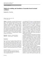
Figure 1.1: Example of two dimensional electron gases (2DEG) on a heterostruc-
ture: The metallic QPC depletes the charges between the source and drain leaving
a Coulomb island quantum dot and the gate can tune the quantum dot occupa-
tions. Discrete quantum channels in the centre region exhibits quantized conduc-
tance as the gate voltage is varied. Conductance quantization was first observed
in GaAlAs-GaAs heterostructures
[
37]
.
the interface with the metal probes. Quantum point contacts (QPC) and molecular
electronics are also particularly described under this category.
The phase coherence of charge carries plays a central part in mesoscopic sys-
tems which often extends over most part of the transport process. This condi-
tion often exhibits interference effects and a host of other interesting phenomena
readily observable in the experiments. The phase coherence can be affected by
external controls such as temperature or any arbitrary time dependent perturba-
tions from external sources like electric or magnetic fields. Some examples for
such phenomena is the universal conductance fluctuation
[
35]

where the conduc-
tance of a sample rapidly changes on the scale of e
2
/h when an external control
parameter is changed. The external parameter could be magnetic field or thermal
cycling and the fluctuations reflect the changes in the conduction channels. This
could be due to different impurity configuration introduced by thermal cycling or
the difference in the way the conduction channels are located in the sample by
the external magnetic field. The weak localization
[36]
is another example where
coherent backscattering by impurities in a certain sample introduces greater re-
sistance to the charge carriers. A typical example relevant to the physical setting
8
1.2. AN OVERVIEW ON QUANTUM TRANSPORT THEORY
above is a mesoscopic junction which consists of a Coulomb island, or a quantum
dot geometrically aligned with a source and drain which may be a 2DEG with a
small gap that allows a finite amount of charge tunneling to and from the quantum
dot. The quantum dot can be tuned by a gate, typically this is a metallic structure
deposited on top of a heterostructure by standard lithography techniques. The
illustration is shown on Fig.
1.1
9
CHAPTER 1. LITERATURE REVIEWS
10
Chapter 2
Theoretical formalisms
Abstract: The chapter serves as a theoretical formalisms to the following three
chapters that would discuss each findings stated in the summary in detail. This
covers Green’s function, density functional theory (DFT) and superconductivity.

2.1 Green’s function for quantum transport
2.1.1 Equilibrium formalisms
Since the complete and rigorous formalisms can be found in many major
texts
[
34,38,39]
, we shall not repeat them all here. Rather, we shall present them
in a summarized form that would be more relevant to our subsequent discussions
later. Therefore the formalism here is only a select few from the literature that are
not meant to be general nor detailed, but only sufficient for our specific purpose.
For simplicity, the formalism would be restricted to fermions at zero temperature.
Basic definitions
Equilibrium Green’s functions are commonly used to calculate scattering like
problems where the particles are initially free, and then they come to interact
for a finite time, after which they scatter apart to free particles again. Thus the
perturbations can be thought of as a switched on-switched off interactions. First,
11
CHAPTER 2. THEORETICAL FORMALISMS
it is our interest to study objects such as,
G(k, t; k
′
, t
′
) = −iη
0
|T {a
k
(t)a
†
k

′
(t
′
)}|η
0
 (2.1)
because experimentally relevant quantities can be extracted easily from such a
mathematical construct, and more importantly, the definition in Eq.(
2.1) allows for
systematic perturbation expansions. The creator and annihilator operators there
are in the Heisenberg’s picture and T is the time ordering operator,
T {a(t)b(t
′
)} = θ(t − t
′
)a(t)b(t
′
) − θ(t
′
− t)b(t
′
)a(t). (2.2)
The Green’s function above is called chronological Green’s function, and the |η
0

are the ground state of the system. Strictly speaking, there should be η
0
|η
0
 as

the denominator of Eq.(
2.1) for normalization and rigorous phase cancelation in
perturbation formalism later but it is neat to suppress them here. For Hamiltoni-
ans linear in number operator, eg. H
0
=Σ
k
ǫ
k
a
†
k
a
k
, we can derive the equation of
motion for the Green’s function,

i
∂
∂t
− ǫ
k

g(k, t; k
′
, t
′
) = δ(t − t
′
)δ

kk
′
(2.3)
which shall make frequent appearance in later discussions. The lower case g in
our convention shall always refer to Green’s function for non-interacting systems
(free propagator) as H
0
above. Other similar Green’s function objects that would
be useful later are,
G
r
(k, t; k
′
, t
′
) = −iθ(t − t
′
){a
k
(t), a
†
k
′
(t
′
)} (2.4)
G
a
(k, t; k
′

, t
′
) = iθ(t
′
− t){a
k
(t), a
†
k
′
(t
′
)} (2.5)
G
<
(k, t; k
′
, t
′
) = ia
†
k
′
(t
′
)a
k
(t) (2.6)
G
>

(k, t; k
′
, t
′
) = −ia
k
(t)a
†
k
′
(t
′
). (2.7)
These functions are interdependent and they are defined for convenience in writ-
ing and evaluating various expressions later. The retarded function (G
r
) is a re-
sponse function at time t due to earlier perturbation at time t
′
, and the advanced
12
2.1. GREEN’S FUNCTION FOR QUANTUM TRANSPORT
function (G
a
) is the response function for the opposite case. Both functions are
often used to calculate spectral properties, density of states or scattering rates. The
lesser function (G
<
) physically represents particle or electron propagator, and the
greater function (G

>
) is the propagator for the anti particles or holes. They contain
information about kinetic properties such as current and particle densities. Their
free propagators can easily be derived from the equation of motion above,
g
r
(k, t − t
′
) = −iθ(t − t
′
)e
−iǫ
k
(t−t
′
)
(2.8)
g
a
(k, t − t
′
) = iθ(t
′
− t)e
−iǫ
k
(t−t
′
)
(2.9)

g
<
(k, t − t
′
) = if(ǫ
k
)e
−iǫ
k
(t−t
′
)
(2.10)
g
>
(k, t − t
′
) = −i (1 − f (ǫ
k
)) e
−iǫ
k
(t−t
′
)
(2.11)
and they are all diagonal in k, and only depends on the time difference as expected
because equilibrium systems are translationally invariant. The function f(ǫ
k
) is

defined as
f(ǫ
k
) =
1
1 + e
β(ǫ
k
−ǫ
F
)
(2.12)
is the usual Fermi Dirac distribution function for electron gas. In the frequency
domain they take the following form,
g(k, ω) =

∞
−∞
d(t − t
′
)e
iω(t−t
′
)
g(k, t − t
′
) (2.13)
and by using the standard complex contour integral we obtain,
g
r

(k, ω) =
1
ω −ǫ
k
+ iη
(2.14)
g
a
(k, ω) =
1
ω −ǫ
k
− iη
(2.15)
g
<
(k, ω) = 2πif(ǫ
k
)δ(ǫ
k
− ω) (2.16)
g
>
(k, ω) = −2πi (1 − f (ǫ
k
)) δ(ǫ
k
− ω) (2.17)
Perturbation expansion
The Hamiltonians to be solved always contain a term V that does not com-

mute with H
0
, and it typically consists of two body operators such as Coulomb
13