Modeling of tumor growth and optimization of therapeutic protocol design
Bạn đang xem bản rút gọn của tài liệu. Xem và tải ngay bản đầy đủ của tài liệu tại đây (4.55 MB, 204 trang )
MODELING OF TUMOR GROWTH AND
OPTIMIZATION OF THERAPEUTIC PROTOCOL
DESIGN
KANCHI LAKSHMI KIRAN
B.E.(Hons), National Institute of Technology, Durgapur, India
A THESIS SUBMITTED
FOR THE DEGREE OF DOCTOR OF PHILOSOPHY
DEPARTMENT OF CHEMICAL & BIOMOLECULAR ENGINEERING
NATIONAL UNIVERSITY OF SINGAPORE
2011
ACKNOWLEDGMENTS
Firstly, I would like to thank my parents for their love and affection, valuable
teachings and their perseverance in making me a responsible global citizen. My
parents have been the prime force behind my achievements. I want to dedicate this
work to my parents. I am thankful to my brothers, uncle and my late grandparents
for their love, concrete support and encouragement.
I am very lucky to be part of the group “Informatics Process Control Unit
(IPCU)” under the supervision of Dr. Lakshminarayanan Samavedham (Laksh). I
would like to thank Dr. Laksh not only for introducing me to an interesting research
discipline but also for his support, encouragement, and mentorship. During my PhD,
I was given complete freedom which provided me more opportunities to learn and
cherish various phases of my graduate student life. I was allowed to teach graduate
and undergraduate students, mentor final year projects of undergraduate students,
attend and organize conferences and meetings and lead the activities of Graduate
Students Association (GSA). My journey of PhD at NUS has been very adventurous
and I feel it is like swimming in an ocean rather than swimming in a pool. I have
got everlasting recipe from the thoughtful discussions with Dr. Laksh on several
topics for leading a fruitful life.
I would like to thank my senior IPCU members - Balaji, Raghu, Sreenu, Sundar
for sharing their invaluable experiences and for their motivation during the budding
stage of my PhD which accelerated my research progress. Also, I would like to
thank my contemporary IPCU members - Abhay, Naviyn, Logu, Karthik, May Su,
Prem, Manoj, Vaibhav, Krishna, Pavan, Kalyan for their professional comments and
critique. I carry with me a lot of happy memories of the IPCU lab.
ii
I would like to thank the department for giving me an opportunity to serve
as the President of GSA - ChBE. I also would like to extend my sincere thanks
to GSA committee members - Sudhir, Sundaramoorthy, Suresh, Abhay, Sadegh,
Naviyn, Logu, Hanifa, Vasanth, Niranjani, Shreenath, Anoop, Ajitha, Vamsi, Anji,
Srivatsan and Vignesh for their support, cooperation and hope on me as a leader.
Moreover, I want to thank all other friends from NUS for their help.
I would like to thank Prof. Farooq and Prof. Feng Si-Shen for their constructive
comments and suggestions on my PhD qualifying report and presentation. I also
want to thank Prof. Krantz, Dr. Rudiyanto Gunawan, Prof. Rangaiah at NUS,
Singapore and Prof. Sundarmoorthy at Pondicherry Engineering college, India for
their help and encouragement.
I wish to thank Prof. Vito Quaranta, Vanderbilt University for providing me
an opportunity to deliver an invited lecture at Vanderbilt Ingram Cancer Centre,
Vanderbilt University.
I would like to thank administrative staff and lab officers of the department for
their help during my PhD.
Last but not least, I am very grateful to NUS for providing me precious moments,
financial support and a platform for participating in various global programs which
led to my allround development.
iii
TABLE OF CONTENTS
Page
Summary . . . . . . . . . . . . . . . . . . . . . . . . . . . . . . . . . . . viii
List of Tables . . . . . . . . . . . . . . . . . . . . . . . . . . . . . . . . . x
List of Figures . . . . . . . . . . . . . . . . . . . . . . . . . . . . . . . . xi
Abbreviations . . . . . . . . . . . . . . . . . . . . . . . . . . . . . . . . . xiv
Nomenclature . . . . . . . . . . . . . . . . . . . . . . . . . . . . . . . . . xv
1 Introduction . . . . . . . . . . . . . . . . . . . . . . . . . . . . . . . . 1
1.1 Motivation . . . . . . . . . . . . . . . . . . . . . . . . . . . . . . . 1
1.1.1 Role of process systems engineering in cancer therapy . . . 3
1.2 Cancer statistics . . . . . . . . . . . . . . . . . . . . . . . . . . . 5
1.3 What is cancer ? . . . . . . . . . . . . . . . . . . . . . . . . . . . 6
1.3.1 Different stages of tumor growth . . . . . . . . . . . . . . . 8
1.4 Clinical phases . . . . . . . . . . . . . . . . . . . . . . . . . . . . 8
1.4.1 Cancer detection . . . . . . . . . . . . . . . . . . . . . . . 9
1.4.2 Cancer diagnosis . . . . . . . . . . . . . . . . . . . . . . . 9
1.4.3 Cancer therapy . . . . . . . . . . . . . . . . . . . . . . . . 10
1.4.4 Emerging and targeted therapies . . . . . . . . . . . . . . 11
1.5 Our focus - avascular tumor growth . . . . . . . . . . . . . . . . . 13
1.6 Contributions . . . . . . . . . . . . . . . . . . . . . . . . . . . . . 14
1.7 Thesis organization . . . . . . . . . . . . . . . . . . . . . . . . . . 15
2 Literature review . . . . . . . . . . . . . . . . . . . . . . . . . . . . . 17
2.1 Mathematical modeling of cancer growth . . . . . . . . . . . . . . 17
2.2 Continuum models . . . . . . . . . . . . . . . . . . . . . . . . . . 20
2.2.1 Homogenous models . . . . . . . . . . . . . . . . . . . . . 21
2.2.2 Heterogenous models . . . . . . . . . . . . . . . . . . . . . 23
2.2.3 Spatio-temporal models . . . . . . . . . . . . . . . . . . . 24
2.2.4 Discrete and hybrid models . . . . . . . . . . . . . . . . . 32
iv
Page
2.2.5 Model calibration . . . . . . . . . . . . . . . . . . . . . . . 33
2.3 Tumor and its interaction with immune system . . . . . . . . . . 34
2.3.1 Tumor-immune models . . . . . . . . . . . . . . . . . . . . 37
2.4 Model-based design of treatment protocols of cancer therapy . . . 38
2.4.1 Pharmacokinetic and pharmacodynamic modeling . . . . . 39
2.4.2 Optimal control theory (OCT) . . . . . . . . . . . . . . . . 40
2.4.3 Description of optimization problem formulation using cancer
therapy models . . . . . . . . . . . . . . . . . . . . . . . . 42
2.5 Challenges in the model-based applications . . . . . . . . . . . . . 44
2.5.1 Description of the strategy implemented in this thesis work 45
3 Mathematical modeling of avascular tumor growth based on dif-
fusion of nutrients and its validation . . . . . . . . . . . . . . . . . 47
3.1 Introduction . . . . . . . . . . . . . . . . . . . . . . . . . . . . . . 47
3.2 The proposed model . . . . . . . . . . . . . . . . . . . . . . . . . 48
3.2.1 Model equations . . . . . . . . . . . . . . . . . . . . . . . 50
3.3 Model solution . . . . . . . . . . . . . . . . . . . . . . . . . . . . 52
3.3.1 Non-dimensionalization of equations . . . . . . . . . . . . 52
3.3.2 Numerical procedure . . . . . . . . . . . . . . . . . . . . . 53
3.4 Model validation and discussion . . . . . . . . . . . . . . . . . . . 54
3.4.1 Validation with in vitro data (Freyer and Sutherland, 1986b) 54
3.4.2 Validation with in vitro data (Sutherland et al., 1986) . . . 59
3.4.3 Comparison with Casciari et al. (1992) model . . . . . . . 64
3.4.4 Comparison with parameters of Gompertzian relation based
on experimental data (Burton, 1966) . . . . . . . . . . . . 65
3.5 Conclusions . . . . . . . . . . . . . . . . . . . . . . . . . . . . . . 66
4 Sequential scheduling of cancer immunotherapy and chemother-
apy using multi-objective optimization . . . . . . . . . . . . . . . 67
4.1 Introduction . . . . . . . . . . . . . . . . . . . . . . . . . . . . . . 67
4.2 Mathematical model . . . . . . . . . . . . . . . . . . . . . . . . . 68
4.3 Multi-objective optimization . . . . . . . . . . . . . . . . . . . . . 71
4.3.1 Non-domination set (Pareto set) . . . . . . . . . . . . . . . 72
4.3.2 NSGA-II . . . . . . . . . . . . . . . . . . . . . . . . . . . . 72
v
Page
4.3.3 Post-Pareto-optimality analysis . . . . . . . . . . . . . . . 74
4.4 Problem formulation . . . . . . . . . . . . . . . . . . . . . . . . . 75
4.4.1 Non-dimensionalization . . . . . . . . . . . . . . . . . . . . 78
4.5 Results and discussion . . . . . . . . . . . . . . . . . . . . . . . . 78
4.5.1 Case 1: Chemotherapy . . . . . . . . . . . . . . . . . . . . 78
4.5.2 Case 2: Immune-chemo combination therapy . . . . . . . . 83
4.6 Conclusions . . . . . . . . . . . . . . . . . . . . . . . . . . . . . . 87
5 Model-based sensitivity analysis and reactive scheduling of den-
dritic cell therapy . . . . . . . . . . . . . . . . . . . . . . . . . . . . 89
5.1 Introduction . . . . . . . . . . . . . . . . . . . . . . . . . . . . . . 89
5.1.1 Dendritic cell therapy . . . . . . . . . . . . . . . . . . . . . 90
5.2 Scheduling under uncertainty . . . . . . . . . . . . . . . . . . . . 91
5.3 Mathematical model . . . . . . . . . . . . . . . . . . . . . . . . . 92
5.4 Global sensitivity analysis . . . . . . . . . . . . . . . . . . . . . . 94
5.4.1 Theoretical formulation of HDMR . . . . . . . . . . . . . . 96
5.4.2 RS-HDMR . . . . . . . . . . . . . . . . . . . . . . . . . . . 97
5.5 Results and discussion . . . . . . . . . . . . . . . . . . . . . . . . 99
5.5.1 Uncertainty and sensitivity analysis using HDMR . . . . . 99
5.5.2 Validation of HDMR results using reactive scheduling . . . 102
5.5.3 Comparison between nominal and reactive schedule for cases
1-3 . . . . . . . . . . . . . . . . . . . . . . . . . . . . . . . 103
5.5.4 Reactive scheduling of combination therapy and dendritic cell
therapy . . . . . . . . . . . . . . . . . . . . . . . . . . . . 106
5.6 Conclusions . . . . . . . . . . . . . . . . . . . . . . . . . . . . . . 110
6 Application of scaling and sensitivity analysis for tumor-immune
model reduction . . . . . . . . . . . . . . . . . . . . . . . . . . . . . 112
6.1 Introduction . . . . . . . . . . . . . . . . . . . . . . . . . . . . . . 112
6.2 Mathematical model . . . . . . . . . . . . . . . . . . . . . . . . . 113
6.3 Scaling analysis . . . . . . . . . . . . . . . . . . . . . . . . . . . . 115
6.3.1 Algorithm . . . . . . . . . . . . . . . . . . . . . . . . . . . 116
6.3.2 Reduced model . . . . . . . . . . . . . . . . . . . . . . . . 117
6.4 Global sensitivity analysis for correlated inputs . . . . . . . . . . 120
vi
Page
6.5 Results and discussion . . . . . . . . . . . . . . . . . . . . . . . . 123
6.5.1 Comparison between original model and reduced model via
theoretical identifiability analysis . . . . . . . . . . . . . . 123
6.5.2 Sensitive parametric groups based on global sensitivity analysis 126
6.5.3 Comparison between original model and reduced model - Pa-
rameter estimation . . . . . . . . . . . . . . . . . . . . . . 130
6.6 Conclusions . . . . . . . . . . . . . . . . . . . . . . . . . . . . . . 133
7 Population based optimal experimental design in cancer diagnosis
and chemotherapy - in silico analysis . . . . . . . . . . . . . . . . 135
7.1 Introduction . . . . . . . . . . . . . . . . . . . . . . . . . . . . . . 135
7.2 Mathematical model . . . . . . . . . . . . . . . . . . . . . . . . . 138
7.3 Population-based studies . . . . . . . . . . . . . . . . . . . . . . . 139
7.3.1 Optimal design of experiments for cancer diagnosis . . . . 139
7.3.2 Optimal design of chemotherapeutic protocol and post-therapy
analysis . . . . . . . . . . . . . . . . . . . . . . . . . . . . 144
7.4 Conclusions . . . . . . . . . . . . . . . . . . . . . . . . . . . . . . 150
8 Conclusions and recommendations for future work . . . . . . . . 152
8.1 Conclusions . . . . . . . . . . . . . . . . . . . . . . . . . . . . . . 152
8.2 Recommendations for future work . . . . . . . . . . . . . . . . . . 157
8.2.1 Validation of the tumor growth models . . . . . . . . . . . 157
8.2.2 Model-based therapeutic design . . . . . . . . . . . . . . . 157
8.2.3 Multiscale modeling . . . . . . . . . . . . . . . . . . . . . 158
8.2.4 Statistical analysis using clinical data of cancer . . . . . . 162
References . . . . . . . . . . . . . . . . . . . . . . . . . . . . . . . . . . . 164
Appendix . . . . . . . . . . . . . . . . . . . . . . . . . . . . . . . . . . . 180
Publications & Presentations . . . . . . . . . . . . . . . . . . . . . . . 181
Curriculum Vitae . . . . . . . . . . . . . . . . . . . . . . . . . . . . . . 183
vii
SUMMARY
Cancer is a leading fatal disease with millions of people falling victim to it every
year. Indeed, the figures are alarming and increasing significantly with each passing
year. Cancer is a complex disease characterized by uncontrolled and unregulated
growth of cells in the body. Cancer growth can be broadly classified into three stages
namely, avascular, angiogenesis and metastasis based on their location and extent
of spread in the body. Mechanisms of cancer growth have been poorly understood
thus far and considerable resources have been committed to elucidate these mech-
anisms and arrive at effective therapeutic strategies that have minimal side effects.
Mathematical modeling can help in the modeling of cancer mechanisms, to propose
and validate hypothesis and to develop therapeutic protocols. This research intends
to contribute to this important area of cancer modeling and treatment.
Among these stages, study of avascular stage is quite relevant to the present
trend of technology development. Many mathematical models have been developed
to comprehend the avascular tumor growth, but the availability of a compendious
model is still elusive. This thesis proposes a simple mechanistic model to explain
the phenomenon of tumor growth observed from the multicellular tumor spheroid
experiments. The main processes incorporated in the mechanistic model for the
avascular tumor growth are diffusion of nutrients through the tumor from the mi-
croenvironment, consumption rate of the nutrients by the cells in the tumor and cell
death by apoptosis and necrosis.
Chemotherapy and immunotherapy are the main focus of this thesis - tumor
growth models are integrated with the pharmacokinetic and pharmacodynamic mod-
els of therapeutic drugs. The integrated model is used to optimize the therapeutic
interventions in order to kill the tumor cells and avert the catastrophic side effects
viii
by effectively leveraging multi-objective optimization and control methods. Further-
more, scaling and sensitivity analysis are applied on the tumor-immune models to
screen the dominating mechanisms affecting the tumor growth. Then, the dominant
mechanisms are used to test out the aspects of intrapatient and interpatient variabil-
ity. Application of reactive scheduling approach is addressed to nullify the effects
of intrapatient variability on the therapeutic outcome. Similarly, population-based
simulation studies are carried out to design diagnostic and therapeutic protocols
and to find the parametric combinations that determine the treatment outcome.
Overall, this thesis showcases the utility and ability of process systems engineering
approaches in improving the cancer diagnosis and treatment.
ix
LIST OF TABLES
Table Page
1.1 Differences between benign and malignant tumors . . . . . . . . . . . 7
3.1 Parameter values . . . . . . . . . . . . . . . . . . . . . . . . . . . . . 55
3.2 Maximum volume of multicellular tumor spheroids at different concen-
trations . . . . . . . . . . . . . . . . . . . . . . . . . . . . . . . . . . 58
3.3 Values of the parameter k
1
of Gompertzian empirical relation . . . . 65
4.1 Parameter values (Kuznetsov et al., 1994; Martin, 1992) . . . . . . . 70
5.1 Parameter values (Piccoli and Castiglione, 2006) . . . . . . . . . . . . 95
5.2 Parameter bounds . . . . . . . . . . . . . . . . . . . . . . . . . . . . 99
5.3 Variation of accuracy with sample size and relative error . . . . . . . 101
5.4 Parameter ranking (R) . . . . . . . . . . . . . . . . . . . . . . . . . . 101
5.5 Variation of key parameters . . . . . . . . . . . . . . . . . . . . . . . 107
6.1 Parameter values . . . . . . . . . . . . . . . . . . . . . . . . . . . . . 116
6.2 Parametric groups . . . . . . . . . . . . . . . . . . . . . . . . . . . . 118
6.3 Values of dimensionless coefficients . . . . . . . . . . . . . . . . . . . 119
6.4 Scale factors of rate of change of the scaled states . . . . . . . . . . . 119
6.5 Relative importance of parameter groups (Π
i
) based on S
p
j
using HDMR
model . . . . . . . . . . . . . . . . . . . . . . . . . . . . . . . . . . . 128
6.6 Structural sensitivity indices (S
a
p
j
) for the key parameters . . . . . . 128
6.7 Comparison of confidence regions between original and reduced models 132
6.8 Closeness between parameter estimates and “true” values . . . . . . . 132
x
LIST OF FIGURES
Figure Page
1.1 Change in death rates of different diseases in US from 1950 to 2003 4
1.2 Clinical phases of cancer treatment . . . . . . . . . . . . . . . . . 9
2.1 Publications on tumor microenvironment during 1995-2008 . . . . 18
2.2 Different spatial scales in tumor growth studies . . . . . . . . . . 20
2.3 Classification of tumor growth models . . . . . . . . . . . . . . . . 21
2.4 Functional models . . . . . . . . . . . . . . . . . . . . . . . . . . . 24
2.5 Classification of immune actions . . . . . . . . . . . . . . . . . . . 35
2.6 Description of different immune actions . . . . . . . . . . . . . . . 37
2.7 Metrics of PK-PD modeling . . . . . . . . . . . . . . . . . . . . . 41
2.8 Strategy followed in this thesis . . . . . . . . . . . . . . . . . . . . 46
3.1 Different zones in avascular tumor growth . . . . . . . . . . . . . 48
3.2 Tumor growth curves of simulated and experimental data at 16.5
mmol/L glucose and 0.28 mmol/L oxygen . . . . . . . . . . . . . 56
3.3 Quiescent and necrotic radius at different tumor radius during its
growth at 16.5 mmol/L glucose and 0.28 mmol/L oxygen . . . . . 56
3.4 Tumor growth curves of simulated and experimental data at 16.5
mmol/L glucose and 0.07 mmol/L oxygen . . . . . . . . . . . . . 57
3.5 Quiescent and necrotic radius at different tumor radius during its
growth at 16.5 mmol/L glucose and 0.07 mmol/L oxygen . . . . . 57
3.6 Profile of partial pressure of oxygen (P O
2
) in the HT29 spheroids
when its diameter is 1039 µm . . . . . . . . . . . . . . . . . . . . 60
3.7 Profile of partial pressure of oxygen (P O
2
) in the HT29 spheroids
when its diameter is 1116 µm . . . . . . . . . . . . . . . . . . . . 60
3.8 Profile of partial pressure of oxygen (P O
2
) in the HT29 spheroids
when its diameter is 1169 µm . . . . . . . . . . . . . . . . . . . . 61
3.9 Profile of partial pressure of oxygen (P O
2
) in the HT29 spheroids
when its diameter is 1415 µm . . . . . . . . . . . . . . . . . . . . 61
3.10 Profile of partial pressure of oxygen (P O
2
) in the HT29 spheroids
when its diameter is 2077µm . . . . . . . . . . . . . . . . . . . . . 62
xi
Figure Page
3.11 Profile of partial pressure of oxygen (P O
2
) in the HT29 spheroids
when its diameter is 2156 µm . . . . . . . . . . . . . . . . . . . . 62
3.12 Profile of partial pressure of oxygen (P O
2
) in the HT29 spheroids
when its diameter is 2314 µm . . . . . . . . . . . . . . . . . . . . 63
3.13 Variation of partial pressure of oxygen (P O
2
) at the centre of the
HT29 spheroids with the increase in its diameter . . . . . . . . . . 63
3.14 Comparison between the proposed model and Casciari et al. (1992)
model on the basis of variation of oxygen concentration at the centre
of the EMT6/Ro spheroids with the increase in its diameter . . . 64
4.1 Schematic representation of NSGA-II . . . . . . . . . . . . . . . . 73
4.2 L
2
norm method . . . . . . . . . . . . . . . . . . . . . . . . . . . 74
4.3 Schematic representation of the problem . . . . . . . . . . . . . . 75
4.4 Comparison between original and non-dimensionalized model . . 79
4.5 Algorithm to find the optimal compromise solution . . . . . . . . 79
4.6 Pareto solutions for the problem formulation for case 1 (i.e. only
chemotherapy) . . . . . . . . . . . . . . . . . . . . . . . . . . . . 80
4.7 Comparison of evolution of states between cluster 1 and cluster 2 81
4.8 Evolution of states corresponding to the proposed treatment protocol
of doxorubicin . . . . . . . . . . . . . . . . . . . . . . . . . . . . 81
4.9 Reduced representation of Pareto solutions for the problem formula-
tion for case 2 (i.e. combination therapy) . . . . . . . . . . . . . . 84
4.10 Treatment protocol corresponding to the proposed combination ther-
apy . . . . . . . . . . . . . . . . . . . . . . . . . . . . . . . . . . 85
4.11 Evolution of states corresponding to the proposed combination ther-
apy . . . . . . . . . . . . . . . . . . . . . . . . . . . . . . . . . . . 85
4.12 Comparison of tumor relapse time between the proposed chemother-
apy and the proposed combination therapy . . . . . . . . . . . . . 86
5.1 Dendritic cell/Vaccine therapy . . . . . . . . . . . . . . . . . . . . 90
5.2 Comparison between nominal and reactive schedule when parameters
are not varied . . . . . . . . . . . . . . . . . . . . . . . . . . . . . 104
5.3 Comparison between nominal and reactive schedule when key param-
eters are varied . . . . . . . . . . . . . . . . . . . . . . . . . . . . 104
5.4 Comparison between nominal and reactive schedule when non-key
parameters are varied . . . . . . . . . . . . . . . . . . . . . . . . . 105
5.5 Comparison of α value for the three cases . . . . . . . . . . . . . . 105
xii
Figure Page
5.6 Evolution of tumor for different therapy cases . . . . . . . . . . . 109
5.7 Reactive schedule of dendritic cell therapy . . . . . . . . . . . . . 109
5.8 Comparison of total dosage between reactive scheduling and nominal
scheduling . . . . . . . . . . . . . . . . . . . . . . . . . . . . . . . 110
6.1 Sequential methodology . . . . . . . . . . . . . . . . . . . . . . . 113
6.2 Comparison of evolution of states between original model and reduced
model . . . . . . . . . . . . . . . . . . . . . . . . . . . . . . . . . 120
6.3 Sensitivity indices of the parametric groups . . . . . . . . . . . . . 126
6.4 Patterns of HDMR component functions with the variations in key
parameters. X-axis: Scaled key parameter values, Y-axis: Scaled
values of the component functions . . . . . . . . . . . . . . . . . . 129
7.1 Determination of diagnostic protocol (D
i
) for a patient population
based on information index (I
i
) evaluated using the mathematical
model . . . . . . . . . . . . . . . . . . . . . . . . . . . . . . . . . 137
7.2 Post - therapy analysis using statistical modeling to find the rules
determining the therapeutic effect on a patient . . . . . . . . . . . 137
7.3 Pareto solution (problem formulation A) corresponding to population
based design of diagnostic protocol . . . . . . . . . . . . . . . . . 143
7.4 Proposed sampling times of tumor, CD8+ T-cells and interleukin
during diagnosis . . . . . . . . . . . . . . . . . . . . . . . . . . . . 143
7.5 Pareto solution (problem formulation B) corresponding to population
based design of treatment protocol . . . . . . . . . . . . . . . . . 146
7.6 Proposed treatment protocol for the considered patient cohort . . 148
7.7 Tumor evolution in different patients . . . . . . . . . . . . . . . . 148
7.8 Rules to determine the success of proposed treatment protocol on the
population . . . . . . . . . . . . . . . . . . . . . . . . . . . . . . . 149
8.1 Application of this thesis work in the clinical practice . . . . . . . 156
8.2 A multiscale framework for comprehending cancer using OMICS data 161
8.3 Identification of diagnostic features and the prediction of therapeutic
design using clinical data . . . . . . . . . . . . . . . . . . . . . . . 162
xiii
ABBREVIATIONS
DZM Different zone model
MZM Mixed zone model
MCTS Multicellular tumor spheroids
MAT Monoclonal antibody therapy
ACT Adoptive-cell-transfer therapy
AUC Area under the curve
PK Pharmacokinetic
PD Pharmacodynamic
OMM Oxygen microelectrode measurements
MOO Multi-objective optimization
GA Genetic algorithm
NSGA Non-dominated sorting genetic algorithm
TRT Tumor relapse time
DC Dendritic cells
DCV Dendritic cell vaccine
GSA Global sensitivity analysis
VBM Variance based methods
HDMR High dimensional model reduction
EFAST Extended fourier amplitude sensitivity tests
RS-HDMR Random sampling - High dimensional model reduction
FIM Fisher information matrix
xiv
NOMENCLATURE
Chapter 2
N Tumor cells
N
0
Initial number of tumor cells
k Proliferation rate constant
θ Carrying capacity of tumor size
α Parameter which determines whether the saturated tumor
size is attained quickly or slowly
P , Q, D Densities of proliferating cells, quiescent cells, dead cells
k
pp
Proliferation rate of proliferating cells
k
pq
, k
qp
, k
pd
, k
qd
Transformation rate constant
λ Decay rate of dead cells
C
i
(r, t) Concentration distribution of the diffusible chemicals
R(t) The position of the outer tumor radius
R
q
(t) The locus of the boundary separating proliferating and qui-
escent cells
R
n
(t) The locus of the boundary separating quiescent and necrotic
cells
D
i
Diffusion coefficient
φ
i
Volume fraction of cell type in a given phase
ν
i
Velocity of cell type in a given phase
λ
i
(φ
i
, C
i
) Chemical and phase dependent production
C(t) Therapeutic drug
X(t) State variables
U(t) input or control or manipulated variables
xv
Chapter 3
C
i
(t) Concentration of nutrients (Oxygen or Glucose)
R(t) The position of the outer tumor radius
R
q
(t) The locus of the boundary separating proliferating and qui-
escent cells
R
n
(t) The locus of the boundary separating quiescent and necrotic
cells
A Proliferation rate constant
A
p
Apoptosis rate constant
N
e
Necrotic rate constant
C
i∞
Concentration of the nutrient at the tumor surface
D
1
Diffusivity of glucose
C
1c
Critical concentration of glucose
µ
1
Maximum consumption rate of glucose
K
1
Michaelis-Menten constant for glucose
D
2
Diffusivity of oxygen
C
2c
Critical concentration of oxygen
µ
2
Maximum consumption rate of oxygen
K
2
Michaelis-Menten constant for oxygen
ν Volume of the tumor
ν
0
Initial volume of the tumor
k
1
, k
2
Gompertzian parameters
Chapter 4
E(t) Effector cells
T (t) Tumor cells
M(t) Chemotherapeutic drug
N Number of therapeutic interventions
t
f
Stipulated course period
xvi
N
e
Number of interventions of effector cells
Chapter 5
H(t) Helper T-cells
C(t) Cytotoxic T-cells
M(t) Tumor cells
D(t) Dendritic cells
I(t) Interleukin
V
f
Variance of the model output
V
i
,V
ij
Partial variances of the inputs
S
i
,S
ij
Sensitivity indices
G Model output
P Parameter set
u
1
Input rate of dendritic cells
u
2
Input rate of interleukin
Chapter 6 & 7
T Tumor cells
N Natural killer cells
L Cytotoxic T-cells
C Circulating lymphocytes
I Interleukin
M Doxorubicin
U Input rate of doxorubicin
O Model output
G
i
Sensitivity matrix
J
c
Joint confidence interval
ψ
1
Significance level
Π
i
Parametric groups
α
i
time derivative scale factors
xvii
T
s
, N
s
, L
s
, C
s
, M
s
Scale factors
n
P 1
, n
P 2
population size
xviii
Chapter 1 Introduction
Chapter 1
INTRODUCTION
‘Growth for the sake of growth is the ideology of the cancer cell.’
- Edward Abbey
1.1 Motivation
The global challenge driving the oncology community is to understand and ex-
ploit the complex nature of cancer growth to discover specific diagnostic indices
and treatment protocols for anti-cancer drugs. This challenge demands conduct-
ing laboratory and clinical experiments for the collection of informative data. The
aggregated knowledge from the experiments and clinical experiences must then be
translated into promising therapies and used in P4 (preventive, proactive, partic-
ipatory and personalized) medicine. Presently, cancer diagnostic and treatment
protocols are suggested based on the knowledge generated from clinical trials in-
volving particular cohort of patients, but are applied on other patient groups as well
(Kleinsmith, 2005). Also, for a given treatment protocol only few patients may be
cured and others may not. Variability in patient outcomes is one of the practical
challenges of the existing and emerging therapeutic protocols. Variability can be
broadly classified as interpatient and intrapatient variability. Interpatient varibility
is the difference in effect of therapy (target or side effects) on different patients. On
the other hand, intrapatient variability is the variations that occur in a given patient
during the treatment course. In fact, it is necessary to know the reason behind the
variability of the effect of diagnostic and treatment protocols on the patients, so
that the protocols can be tailored appropriately to individual patients or patient
1
1.1 Motivation
groups. It is to be noted that experiments that can elucidate the reasons for inter-
and intrapatient variability are costly and time-consuming. The objectives of any
therapy are to minimize the total number of cancer cells by maintaining it below
the lethal level while minimizing the side effects. Keeping this in view, the main
challenge is to find a way for the clinical implementation of novel and combinatorial
therapies. FDA approval is needed before any clinical implementation - the whole
process of discovery, laboratory trials and approval can take several years. Accord-
ing to recent studies, the cost involved in the research and development of a new
drug for Food and Drug Administration (FDA) approval is between US $ 500 million
and US $ 800 million and the development time is around 10-12 years. For example,
Dendreon took around 18 years to get FDA’s approval and around US $ 750 million
was invested. A lot of in vitro/in vivo experiments should be performed to clear
the different phases of FDA approval and understand the side effects, efficacy and
the variability of the therapy (Lord and Ashworth, 2010). In this context, in silico
(computer) based tools may help to investigate the fundamentals of cancer growth
and unique features of a given therapy and its protocols. Even FDA has recognized
and encouraged the population based pharmacokinetic and pharmacodynamic mod-
eling studies to ease the approval of new drugs with lesser number of experiments.
In this regard, Gatenby (1998) states that ‘recent research in tumor biology, partic-
ularly that using new techniques from molecular biology, has produced information
at an explosive pace. Yet, a conceptual framework within which all these new (and
old data) can be fitted is lacking’. Gatenby and Gawlinski (2003) stress the point
that clinical oncologists and tumor biologists possess virtually no comprehensive
theoretical model to serve as a framework for understanding, organizing and apply-
ing the data and emphasize the need to develop mechanistic models that provide
real insights into critical parameters that control system dynamics. Murray (2002)
states that ‘the goal is to develop models which capture the essence of various in-
teractions allowing their outcome to be more fully understood’. Tiina et al. (2007)
presented the results of a search in the PubMed bibliographic database which shows
2
Chapter 1 Introduction
that, out of 1.5 million papers in the area of cancer research, approximately 5% are
related to mathematical modeling. According to Byrne (1999), effective and efficient
treatment modalities can be developed by identifying the mechanisms which control
the cancer growth. Thus, once we understand the mechanism, the key components
of it can be modified to eliminate (or reduce pain arising from) the disease. This
state of knowledge may be possibly reached through laboratory experiments alone,
but at the cost of infinite time and numerous (replicated) experiments. However,
the achievement of this goal can be speeded up through the application of process
systems engineering techniques (Mathematical modeling, Control theory and Op-
timization) to describe different aspects of solid tumor growth in the absence or
presence of anti-cancer agents. This implies that sound and robust tools are essen-
tial in order to investigate the fundamentals of cancer growth and unique features
of a given therapy and its protocols.
1.1.1 Role of process systems engineering in cancer therapy
Mathematical modeling and simulation is a versatile tool in comprehending the
system behavior and has been used for different applications in natural science and
engineering disciplines (Quarteroni, 2009). A mathematical model is an abstraction
of a process system. It is composed of model equations and parameters. Usually,
available experimental data is used for estimating the model parameters and for val-
idating its prognostic ability. Then, parametric analysis (sensitivity analysis with
respect to parameters) of the model is performed to understand the domain and
variations of the system behavior with the variation in the parameters (Rodrigues
and Minceva, 2005). With understanding of the system and a valid model, one can
pursue model based process control and optimization (Edgar et al., 2001). In a sim-
ilar fashion, the applications of the tumor growth modeling are many (Deisboeck
et al., 2009). Firstly, cancer growth can be predicted and the main parameters re-
sponsible for it can be better understood. Secondly, these models can be combined
3
1.2 Cancer statistics
with pharmacokinetic and pharmacodynamic models of the therapeutic agents to
study their impact on cancer growth (Quaranta et al., 2005). Thus, the combina-
tion model can serve as a decision-making tool for planning and scheduling of the
different therapies. In addition, interpatient and intrapatient variability scenarios
can be imitated by perturbing the parameters and optimization techniques can be
used to schedule a therapy accordingly. Modeling and in silico experiments can
provide new insights and offer different possibilities to understand and treat can-
cer. Experimentalists and clinicians are becoming increasingly aware of the role of
mathematical modeling and its value-addition along with medical techniques and
experimental approaches in order to accelerate our understanding in distinguishing
various possible mechanisms responsible for the tumor growth (Friedrich et al., 2007;
Gottfried et al., 2006; Kunz-Schughart et al., 1998; Kunz-Schughart, 1999; Oswald
et al., 2007).
Fig. 1.1. Change in death rates of different diseases in US from 1950 to 2003
4
Chapter 1 Introduction
1.2 Cancer statistics
The word Cancer (meaning “crab” in Latin) was introduced by Hippocrates in
the 5
th
century BC to explain a group of diseases resulting from the abnormal growth
and spread of tissues to the other parts of the body and ultimately proving fatal.
Even though cancer has subsisted for a very long time, its existence is noticeably
increasing during the last 50 years. As of now, the probability that a randomly
selected person will get cancer has almost doubled when compared to 1950s (Klein-
smith, 2005). Cancer stands next only to heart disease in the list of most fatal
diseases in the world. From Figure 1.1, it is obvious that the decrease in death rate
of cancer patients over the years 1950-2003 has been minimal as compared to other
major diseases. Cancer related deaths have been escalating meteorically - according
to the World Health Organization (WHO), 7.6 million people died of cancer (out of
58 million deaths overall) in 2008. They speculated that cancer deaths will increase
to 18% and 50% by 2015 and 2030 respectively. Recently, the American Cancer
Society (ACS) reported that around 1.6 million new cancer cases and 0.6 million
cancer death cases occured in the US in 2009. According to another report on
worldwide cancer rates by the WHO’s International Agency for Research on Cancer
(IARC), North America leads the world in the rate of cancers diagnosed in adults,
followed closely by Western Europe, Australia and New Zealand. In Britain, it was
estimated using 2008 data that more than one in three were expected to develop
the disease over their survival period
1
. According to Cancer Council Australia,
around 114,000 new cases of cancer were diagnosed in Australia in 2010 and it was
estimated that one in two Australians will be diagnosed of cancer by the age of 85.
Cancer deaths in Singapore reflected the global trend (27.1% of total deaths) during
the period 1998-2002 and approximately 49,400 new cases of cancer were diagnosed
during the period 2005-2009
2
. The reasons for such alarming trends include the
1
/>2
Trends Report%20 05-09.pdf
5
1.3 What is cancer ?
non-availability of definite therapy for all types of cancer and the indeterminate
nature of the existing therapies for patients with same type of cancer.
The above mentioned figures have drawn the attention of researchers to under-
stand the mechanism of cancer and come out with better therapies. In this effort,
remarkable progress has been made in the past few decades in uncovering some of
the cellular and molecular mechanisms leading to cancer and the cumulative infor-
mation reveal that around 100 types of cancer exist. Their names are distinguished
from one another on the basis of its location and the cell type involved. Based on
the gravity of the cancer problem, Perumpanani (1996) remarks that ‘the research
community has taken on the challenge posed by cancer on a war-footing and this
has in recent years resulted in an explosion in our understanding of cancer’. Some
researchers claim that the analysis of cancer mechanisms has enhanced our under-
standing of the normal cells (Alberts et al., 2002; Kleinsmith, 2005). This may
lead to many fundamental discoveries in cell biology and broadly benefit the vari-
ous fields of medicine. Despite the advances made in the understanding of cancer
and mechanisms, much remains to be done before the deaths of millions of people
due to cancer can be reduced. One main challenge is to be able to understand and
exploit the complex nature and multiple stages of tumor growth. Another challenge
is to conduct the right laboratory and bedside experiments to collect useful data to
extract information regarding the mechanisms of cancer cell behavior.
1.3 What is cancer ?
Cancer is the uncontrolled proliferation of abnormal cells of any tissue or organ
in the human body. An abnormal cancer cell evolves from the normal cell due to
accumulation of DNA damage - this DNA damage (i.e. genetic mutations in pieces of
DNA) makes the cell immortal. The genes transferred from the parents might carry
with them an inherent risk or susceptibility to cancer. When such a “normal” but
6
Chapter 1 Introduction
Table 1.1
Differences between benign and malignant tumors
Trait Benign Malignant
Nuclear size Small Large
Ratio of nuclear size to Low High
cytoplasmic volume
Nuclear shape Regular Pleomorphic (irregular shape)
Mitotic index Low High
Tissue organization Normal Disorganized
Differentiation Well differentiated Poorly differentiated
Tumor boundary Well defined Poorly defined
“risk prone” cell is exposed to external factors such as UV radiation, carcinogenic
chemicals etc., it could undergo a series of genetic mutations and transform into a
cancerous cell. Mutations cause the cell to evade cell death and grow improperly
with or without growth signals from the environment (Hanahan and Weinberg, 2000;
Martins et al., 2007). Once the cancer cell is formed, it searches for nutrients from
the nearby tissues and proliferates rapidly compared to the adjacent normal cells
(Tiina et al., 2007). The induced mutation by the external factors not only enhances
the proliferation rate of the cells but also decreases its death rate by down-regulating
and up-regulating the tumor suppressor genes and oncogenes respectively (Hanahan
and Weinberg, 2000). Over time, this results in the formation of a clump of cells
known as neoplasm or tumor. Tumor growth is based upon conditions like tumor
location, cell type, and nutrient supply. On the basis of the growth pattern, tumors
are classified into two fundamental groups. One group is benign tumors whose
growth is narrowed to a local area and are composed of well-differentiated cells.
The other one is malignant tumors which can invade the nearby tissues, migrate to
other parts of the body and their cells are poorly differentiated. The differences in
the microscopic appearance of the benign and malignant tumors are tabulated in
Table 1.1.
7