Thermal combustion and oxygen chemisorption of wood exposed to low temperature long term heating 2
Bạn đang xem bản rút gọn của tài liệu. Xem và tải ngay bản đầy đủ của tài liệu tại đây (132.32 KB, 28 trang )
Chapter 2: Literature Review
________________________________________________________________________
26
Chapter Two: Literature Review
2 Introduction
The heating of wood involves physical changes such as enthalpy and moisture
content. One of the major links between temperature and moisture changes is water
evaporation. Water evaporation acts as a heat source term in the energy balance, and
contributes to physical processes of heat and mass transfer in the heating of wood. This
chapter reviews first the chemical changes i.e. pyrolysis and physical processes of heat
and mass transfer within the framework of wood combustion so that any addition,
alteration and omission of physical variables in the mathematical formulation could be
better understood in terms of its impact. Because water evaporation is an important link
in wood heating, the different formulations on modeling of evaporation in wood heating
are also reviewed. The objective is to elucidate the most optimum way to represent this
physical process in the modelling of wood heating and combustion, when the evaporation
front has recessed into wood.
There have been different modeling approaches towards evaporation in wood heating.
Using one approach instead of the other represents a different understanding to the
physical process of evaporation in wood drying. Water evaporation in hygroscopic wood
is primarily concerned with the changes in equilibrium pressure of water vapour with
temperature and moisture content; this chapter hence first reviews the equilibrium and the
Chapter 2: Literature Review
________________________________________________________________________
27
non-equilibrium approaches. The different principles and formulations are discussed, and
the problems for applications in wood heating are evaluated with respect to both low-
temperature and high-temperature drying. Alternative approaches such as the desorption
kinetics approach and the evaporation temperature approach are also discussed.
2.1 Reviews of physical and chemical studies in wood combustion
Combustion is a complex problem involving solid-phase and gas-phase
phenomena. For bench-scale methods such as Cone Calorimeter, analysis is mainly on
solid-phase phenomena; gas-phase diffusion and chemical kinetics are relatively
unimportant for this scale of evaluation, involving less complex geometry (Janssens
1991a). Chemical reaction and the heat and mass transfer processes constitute a complete
solid-phase phenomenon. Chemical and physical processes however do not play equal
parts in thermal model. This review considers a comprehensive combustion model that
includes pyrolysis as well as heat and mass transfer in the formulation of a mathematical
model.
2.1.1 Heat and mass transfer in solid phase
In pure thermal models, heat transfer is solely accounted by conduction. The flow
of pyrolysate gases (henceforth known as “volatiles”) is not considered in the energy
equation. In the respective one-dimensional and three-dimensional model of Bamford et
al. (1946) and Bonnefoy et al. (1993), their energy equation contains a heat diffusion
Chapter 2: Literature Review
________________________________________________________________________
28
term with thermal decomposition described by a first-order Arrhenius equation, acting as
a heat source term. The convective heat transfer due to the flow of volatiles was not
included. Such pure thermal models are often employed to limit the problems as a
conduction case, so that useful insights could be obtained to form analytical solutions.
Janssens (1993) has used a thermal model to successfully correlate ignition with thermal
properties of wood slabs. Besides, pure conduction problems are also widely used to
study ignition in materials that are irradiated on one side and lose heat by Newtonian
cooling (Simms 1960).
There came the findings from Kanury and Blackshear (1970a and 1970b). They studied
the convection of volatiles in a pyrolysing solid and demonstrated the importance of
internal convection to the overall heat balance. They examined the relative magnitude of
convection term to conduction term, and showed that the Peclet number is greater than
0.1. Peclet number is a dimensionless number used in calculations involving convective
heat transfer; it is the ratio of thermal energy convected to the fluid to the thermal energy
conducted within the fluid. Peclet number is in fact a product of Reynolds number and
Prandtl number, which can be expressed as
2
10 10
( )/ ( )/
p
CV TT lkTT l
ρ
∞
∗∗∗− ∗−
. The
finding that Peclet number was greater than 0.1 in this case strongly endorsed the
significance of internal convective heat transfer. In addition, their research further
pointed out that the effect of convection would increase in tandem with the corresponding
increase in specimen’s size. Internal convection of volatiles was subsequently included in
the energy equation of many pyrolysis models (Kanury and Blackshear 1970b, Kung
1972, Kung and Kalelkar 1973, Kansa, Perlee and Chaiken 1977, Boonmee 2004). The
Chapter 2: Literature Review
________________________________________________________________________
29
energy transport equations in these works however did not include a convective heat
transfer term for the flow of water vapour; moisture was either not considered, or not
treated explicitly. Kung (1972) discussed the significance of both the outward
convection of volatiles and char conductivity on the pyrolysis wave propagation, but did
not consider the evaporation of moisture in wood. Kansa et al (1977) incorporated the
momentum equation for the movement of volatiles in solid but not one for volatiles.
Boonmee (2004) considered the effect of water vaporisation to be insignificant in the
case of oven-dry wood and ignored convection of vapour on heat transfer.
Vapour was added to the energy equation in some models on the ground that the
vaporisation could be significant on the overall heat balance. Chan et al (1985), Fredlund
(1988), Alves and Figueiredo (1989) and Yuen (1998) have included moisture
evaporation as an additional heat source term, treating the latent heat of evaporation as
heat of reaction. Convective heat transfer due to vapour was also added alongside
convection of volatiles in the energy transport equation. The inclusion of moisture
evaporation as a heat source term creates a heat sink in the energy balance as it draws
heat from inside the solid to vaporise the moisture. Zhang and Datta (2004) showed that
the conventional treatment of moisture evaporation as a heat source term could create
problems for low rate drying or low heating of wood. The heat sink effect by moisture
evaporation causes the temperature to fall below the actual temperature where the initial
temperature remains fairly constant for initial drying.
Chapter 2: Literature Review
________________________________________________________________________
30
For models that accounted for the production of volatiles, alone or in combination with
water vapours, many of these models (Kung 1972, Kung and Kalelkar 1973, Kansa et al
1977, Chan et al 1985, Boonmee 2004) have assumed that these volatiles and vapours
escape instantaneously to the surface once they are formed. In doing so, these models
have assumed, as well as limited, the flow of volatiles and vapour strictly in the
longitudinal direction, since wood has a large permeability along grain, of which the ratio
of axial to transverse permeability for softwoods is approximately 20,000 (Siau 1984);
the large axial permeability permits relative ease of escape. The velocity of the volatiles
and vapour are given by the flow field which of course has to satisfy the continuity
equation. There is no accumulation of volatiles and vapour, thereby eliminating
accumulation term in the continuity equation. Since it is not a pressure-driven flow,
pressure is assumed constant. Such simplification in mass transfer is often made so that
analytical models ascribed to certain complex combustion phenomenon can be made
tractable (Boonmee 2004).
Driving forces sometimes arise naturally in cases where there is a steep pressure build-up
resulting in a pressure gradient, or concentration difference that promotes diffusion. In
both Fredlund’s model (1993) and Yuen’s model (1998), a pressure equation is provided
as a driving force. In their models, mass transfer of volatiles and vapour is based on gas
flows driven by pressure gradients, the flow of which conforms to Darcy’s law. Both
models allow the pressure to change with porosity of the wood slab, thereby creating the
pressure in the system. The total pressure is then obtained according to Dalton’s law as
the sum of the partial pressures of water vapour and volatiles. Mass source terms are
Chapter 2: Literature Review
________________________________________________________________________
31
created in the continuity equation to allow accumulation of volatiles and evaporation of
vapour. The only difference between the two mass transfer models is that in Fredlund’s
work, additional pressure changes arising from elevating temperature that cause gases to
expand in a constant volume according to the universal gas law have been provided for.
Nonetheless, this additional pressure term is small as compared to pressure change
arising from vaporisation of water in rapid heating rates. In the latter, rapid vaporisation
results in steep pressure gradient.
In both Fredlund’s and Yuen’s models, moisture flow takes place mainly in vapour phase.
Moisture flow can occur in liquid phase, but Fredlund and Yuen have both adopted the
high-temperature drying model proposed by Alves and Figueiredo (1989) which ignored
free water movement. The same assumption of eliminating free water movement has also
been adopted in all the foregoing models that do not use pressure-driven flow. For vapour
and volatiles transport, all models have implicitly (those with pressure driven flow) and
explicitly (those do not employ pressure-driven flow) excluded vapour diffusion. The
assumption that water vapour/ carrier gas diffusion is much slower than vapour
convection reduces the model validity to high-temperature drying i.e. above water boiling
point.
2.2 Evaporation zone in drying model
Modelling of internal evaporation rate will be needed when internal evaporation is
significant, such as when there is an evaporation zone inside the material. It occurs at a
Chapter 2: Literature Review
________________________________________________________________________
32
later stage of drying when diffusivity of liquid becomes small due to diminishing
moisture content. The escaping water flux through the surface decreases, resulting in a
drier surface and a decreasing surface evaporation rate. Eventually, the evaporation front
moves inwards.
Figure 2.1 shows a conceptual model of high-temperature drying in wood where
evaporation zone has retreated inwards, creating an evaporation zone within the
pyrolysing wood (Stanish, Schajer and Kayihan 1986, Farid 2002). Evaporation takes
place in this evaporation zone since it is the location where there is the largest moisture
gradient (Ilic and Turner 1986). The water vapour partly migrates towards and escapes
through the exposed surface. A fraction also migrates in the opposite direction, and re-
condenses at a colder inner region. This high-temperature drying model also models the
formation of cracks and fissures at the char surface, since high-temperature drying occurs
just incipient of or in tandem with flaming combustion. The formation of cracks and
fissures greatly affects the heat and mass transfer between flame and the solid, and hence
the equilibrium of vapour pressure profile at the surface.
Chapter 2: Literature Review
________________________________________________________________________
33
Figure 2.1: Conceptual model of high-temperature drying in wood
(Drying model adapted from Janssens 2004, ©Fire and Materials)
The rate at which the evaporation zone moves into the solid can be calculated by heat
conduction (Williams, 1953). The method divides the solid into two regions separated by
an isothermal plane – the 100°C plateau, the plane of vaporisation. The rate at which this
plane moves at any depth
r
is assumed to depend only upon the net rate of heat transfer
by conduction to that depth. The equation for calculating
r
at time
t
is given by
1/2
1/2
()
constant
2( )
tr
ierfc
kt
λ
β
λ
=
(2.1)
where
λ
is the thermal diffusivity,
k
the thermal conductivity and
ierfc
β
is given as
1. Wet wood
2. Evaporation zone
3. Dry wood
4. Pyrolysis zone
5. Char layer
6. Initial location of
exposed surface
7. Flame
3
Heat transfer
1
2
3
4
5
6
7
Fire
Mass and enthalpy
transfer
Vapour
movement
Pyrolysate
movement
Chapter 2: Literature Review
________________________________________________________________________
34
2
2
exp( )
z
ierfc z dz
β
β
β
π
∞
= −
∫∫
(2.2)
Figure 2.2 shows the depth
()r
of the plane of vaporisation (interface B) calculated by the
heat conduction method. It has been pointed out that in hygroscopic materials, there is no
abrupt interface between the dry zone (Zone A) and the wet zone (Zone C) (Schrader and
Litchfield 1992). The capillary effect still causes water diffusion and vapour generation
depends on moisture content (X) and temperature (T). So, evaporation takes place in a
zone instead of on a sharp interface as shown as “interface B” in Figure 2.2.
Figure 2.2. Evaporation front calculated by heat conduction in high-temperature
drying
(Simplified model of high-temperature drying reproduced from Alves and Figueiredo
1989, ©Chemical Engineering Science)
Incorporating the evaporation zone, instead of an evaporation front into a drying model
yields a high-temperature drying model that has been widely used in pyrolysis studies of
wood. It has thus been commonly referred to as the “conventional high-temperature
T=T
∞
X= 0
Zone A
Zone C
X = constant > 0
Interface B
T=T
ev
r
Chapter 2: Literature Review
________________________________________________________________________
35
drying model” (See Figure 2.3). Vapours are generated in Zone B (evaporation zone)
when temperature reaches the moisture boiling point, or evaporation temperature.
Janssens (2004) pointed out that since water is adsorbed to cell walls, evaporation
requires more energy than needed to boil free water and may occur at temperatures
exceeding 100°C. Alves and Figueiredo (1989) proposed that the evaporation
temperature is governed by the moisture content (X) on dry basis. For 1% < X < 14%, the
evaporation temperature is given as
[ ] [ ]
{ }
23
34 6 5
( ) 1/ 2.13 10 2.778 10 ln( ) 9.997 10 ln( ) 1.461 10 ln( )
ev
TX X X X
−− − −
= ×+× +× −×
(2.3)
Yuen (1998) suggested that when the moisture content in wood is less than 1%, the
evaporation temperature may be assumed to be 473K. For wood with moisture content >
14%, the evaporation temperature can be assumed to occur at 373K, with negligible
discontinuity and error (Alves and Figueiredo, 1989; Yuen, 1998).
Chapter 2: Literature Review
________________________________________________________________________
36
Figure 2.3: Conventional high-temperature drying model
(Drying model reproduced from Alves et al 1989, ©Chemical Engineering Science)
2.3 Formulation of evaporation rate
To include evaporation as an internal term in a drying model, there is a need to
describe the rate of evaporation
ev
R
in the model, through the time to reach equilibrium
between liquid and vapour. Equilibrium approach assumes that equilibrium between
water and vapour is reached instantaneously; the rate of evaporation is formulated with a
known vapour pressure
v
p
. Non-equilibrium approach on the other hand does not assume
water vapour to be in equilibrium with liquid water; vapour pressure remains an unknown
variable. Non-equilibrium approach needs both the equilibrium vapour pressure and the
parameter indicating the rate of evaporation.
Zone A
X = 0
Zone B
T = T
ev
Evaporation
is function
of available
heat
Zone C
T< T
ev
T
ev
(X)
Vapour convection
without resistance
X = constant
Heat transfer
Heated boundary
Symmetry axis or
plane
Chapter 2: Literature Review
________________________________________________________________________
37
2.4 Equilibrium approach
Equilibrium approach assumes that vapour and water are in phase equilibrium at
any time (Plumb, Spolek and Olmstead 1985, Stanish et al. 1986, Crapsite, Whitaker and
Rotstein 1988, Ni, Datta and Torrance 1999). According to ideal gas law, the amount of
vapour per unit volume
V
is given by
vv
pM
V
RT
=
(2.4)
In equilibrium approach, vapour pressure is fixed so long as temperature and/or water
content are given, where
(, )
vv
p p TW
=
(2.5)
Vapour pressure is related to the saturated vapour pressure by water activity
aw
,
(, )
(, )
()
v
v sat
p TW
aw f T W
pT
≡=
(2.6)
where
(, )
v
p TW
is the equilibrium vapour pressure and
,
()
v sat
pT
is the saturated vapour
pressure of water at temperature
T
. There are several formulations of the saturation
vapour pressure. Sahota (1979) used an exponential function to relate the saturation
vapour pressure to temperature
Chapter 2: Literature Review
________________________________________________________________________
38
/
,
exp( )
v
BR
v sat
v
A
p CT
RT
−
−
=
(2.7)
where
31
3.18 10 kJ kgA
−
= ×
,
11
2.5kJ kg KB
−−
=
and
26 2
6.05 10 NmC
−
= ×
. Fredlund
(1988) also proposed that the saturation vapour pressure follows an exponential function
of the thermodynamic temperature of solid
()
s
T
as
,1 2
exp( / )
v sat s
p K KT= −
(2.8)
where
1
K
and
2
K
are constants which depend on the temperature range,
and
10
1
4.143 10K = ×
Pa and
2
4822KK=
in the temperature range of 20°C to 1000°C.
The assumption that vaporization is sufficiently rapid for complete saturation of vapour
in the pores – so long as there is water in the liquid phase at the point of consideration –
further simplifies the relations between
v
p
and
,v sat
p
set out in Equation (2.6), so that
,v v sat
pp=
(2.9)
By determining the vapour pressure,
V
or
v
p
is no longer an independent variable in the
system of conservation equations. The rate of evaporation can be formulated from the
continuity equation and readily solved given the known state variables such as
temperature and pressure distribution. In Yuen (1998) three-dimensional model of
Chapter 2: Literature Review
________________________________________________________________________
39
pressure-driven flows, the rate of evaporation
ev
R
, expressed in the continuity equation,
requires the solution of total pressure inside the system where
xyz
v svs svs svs
ev
ttt
mp mp mp
R
tx x y y z z
ρρ ρ ρ
ρρρ
∂∂ ∂ ∂
∂∂∂
=−−−
∂∂ ∂ ∂ ∂ ∂ ∂
(2.10)
where
t
ρ
is the total sum of the mass of volatile gases, vapour and dry air per unit
volume and
/
jj
s st
mD
η
=
is the respective mass transfer coefficients of the solid as
,,j xyz=
directions;
t
η
being the kinematic viscosity of gaseous mixture in the solid. In
Yuen’s model, the total pressure
s
p
is readily obtained according to Dalton’s law as the
sum of partial pressures of vapour, volatiles and dry air, i.e.
s gvi
pppp= ++
. Alves and
Figueiredo (1989) also formulated the rate of evaporation assuming local moisture-
vapour equilibrium from their heating model which does not consider mass transfer. The
rate of evaporation
ev
R
is formulated from their one-dimensional energy balance
comprising of a thermal decomposition scheme of six constituent components where
1,2 6j =
as follow:
6
()
1
()
ss mm s s
ev s
ev
gg vv ii s
pj pj
j
C CT T
Rk
H t xx
m C mC mC T
HR
x
ρρ
∂+ ∂
∂
= +
∆ ∂ ∂∂
∂ ++
− −∆
∂
∑
(2.11)
Chapter 2: Literature Review
________________________________________________________________________
40
Despite the assumption that the equilibrium between water and vapour pressure is
reached instantaneously, the actual rate of evaporation itself may not be fast enough in
the context of a fast heating scenario. It has been shown that when a piece of material is
put into a closed chamber to measure its water activity
()aw
, it takes two to thirty hours
for the sample to reach equilibrium (Ramanathan and Cenkowski 1995). This is
particularly true when considering dry wood because the strong attraction of water to the
solid matrix (Janssens, 1993) may cause it to take a longer time before the balance can be
established. It probably will be faster for a wet wood to reach equilibrium than a dry one
due to the presence of more free water and the presence of smaller gas bubbles in wet
porous structures (Zhang and Datta, 2004). Transport will also affect the establishment
of equilibrium especially in the dry zone near the surface (Zhang 2003). In the location
near the surface, the vapour convects without much resistance, owing to the formation of
cracks and fissures (see Figure 2.1 and “Zone A” in Figure 2.3). If vapour is lost quickly,
the vapour pressure will be lower than the equilibrium pressure, unless evaporation is
very fast.
It therefore may not be mathematically appropriate to compute the rate of evaporation
directly through the continuity equations assuming the equilibrium approach, because of
the discrepancy between the actual rate of evaporation and the assumption of
instantaneous equilibrium. Besides, the rate of evaporation
ev
R
formulated through the
continuity equations contains the second derivative of the state variables such as
temperature
()T
, pressure
()
s
p
and mass fluxes of respective species. The computational
solution of
ev
R
through the systems of equations will be two orders lower in precision
Chapter 2: Literature Review
________________________________________________________________________
41
(Zhang and Datta, 2004). To overcome the problem, it has been proposed that the
evaporation term is removed from the continuity equations (i.e.
ev
R
is not to be resolved
from the formulation using continuity equation), and to compute the evaporation rate
directly from the systems of modified conservation equations (Zhang, 2003). For instance,
given an one-dimensional system considering water and vapour diffusion, the continuity
equations may be expressed as
()
v ev
VV
DR
tx x
∂∂∂
= +
∂∂ ∂
(2.12)
()
w ev
WW
DR
tx x
∂∂∂
= −
∂∂ ∂
(2.13)
The continuity equations of (2.11) and (2.12) may be combined so that
ev
R
is removed.
The conservation model then consists of two equations:
( )( )
wv
WV
DW DV
tt
∂∂
+ =∇⋅ ∇ +∇⋅ ∇
∂∂
(2.14)
() ( )
ev w
TW
c kT H D W
tt
ρ
∂∂
=∇⋅ ∇ −∆ − +∇⋅ ∇
∂∂
(2.15)
where
()
ev w
W
R DW
t
∂
= − +∇⋅ ∇
∂
in Equation (2.15) which can be obtained from
Equation (2.11). The conservation model is solved directly by replacing variables
Chapter 2: Literature Review
________________________________________________________________________
42
/Vt∂∂
and
V∇
with state variables
T
and
W
through differentiating the ideal gas law
in Equation (2.4), so that
2
2
v v vv
v v v vv
M p pM
V
t RT t RT
M p p pM
TW T
RT T t W t RT t
∂
∂
= −
∂∂
∂∂
∂∂ ∂
= +−
∂∂ ∂ ∂ ∂
(2.16)
2
2
v vv
v
v v v vv
M pM
Vp T
RT RT
M p p pM
TW T
RT t W RT
∇= ∇− ∇
∂∂
= ∇+ ∇ − ∇
∂∂
(2.17)
The substitution of
/Vt∂∂
and
V∇
using Equations (2.16) and (2.17) eliminates the
second derivatives of
T
and
W
from the conservation equations. It thus prevents the
computational errors associated with the second order of differentiation for computing
evaporation rate.
2.5 Non-equilibrium approach
In non-equilibrium approach, it does not assume water vapour is in equilibrium
with liquid water. Indeed, how fast water-vapour can reach equilibrium, or how fast the
evaporation is, needs to be quantified. The rate limit of evaporation and the attainment of
equilibrium are determined by the evaporation rate, either empirically derived or
experimentally quantified.
Chapter 2: Literature Review
________________________________________________________________________
43
How fast evaporation is can be related to the difference between equilibrium vapour
pressure and the actual local vapour pressure. In addition, evaporation rate also depends
on the water content in the material. Bixler (1985) proposed the following evaporation
rate for the non-equilibrium condition:
0 ,*
( )( )
ev v eqb v
R cW W p p=−−
(2.18)
where
W
is the moisture content,
0
W
is the residual moisture content after which the
moisture content does not decrease anymore.
c
is a coefficient that varies with
temperature and moisture content; it should be chosen such that the rate of mass loss
obtained from simulation matches the mass loss in the experiment (Bixler, 1985).
The formulation of evaporation rate such as that in Equation (2.18) is advocated for more
realistic representation of heating in hygroscopic materials (Zhang, 2003). Indeed,
equilibrium approach is considered a special case within the domain of the non-
equilibrium approach. However, there are several difficulties associated with the use of
non-equilibrium approach. The measurement of evaporation is difficult in porous media,
only empirical parameters with unverified accuracy have been used so far (Bixler, 1985).
Besides, in the numerical modeling of porous media, the sharp change of vapour pressure
near the surface causes some numerical difficulty. Zhang (2003) pointed out that the
finite element mesh near the surface needs to be very fine to reach convergence. However,
there is a limit as how fine the mesh size can be reduced to match the pore size since a
valid continuum assumption requires that the size of the Representative Elementary
Chapter 2: Literature Review
________________________________________________________________________
44
Volume (REV) required for building the governing equations is at least a few times larger
than the pore size. Zhang and Datta (2004) indeed argued that since evaporation rate is
not perfect and the knowledge of equilibrium rate remains largely qualitative, there is no
need to pursue exact match between simulation and experiment. Nonetheless, despite the
arbitrary nature of parameters and the formulation of the rate of evaporation, the non-
equilibrium approach is still more realistic than simply ignoring the transition from non-
equilibrium to equilibrium in certain applications (Vafai and Hadim 2000).
2.6 Desorption kinetics approach
Other than the non-equilibrium approach, the desorption kinetics approach is
another alternative approach intended to address the limitations faced in assuming phase
equilibrium between water and vapour throughout the material. Because of the lack of
equilibrium at the surface due to convective removal of vapour, using the equilibrium
vapour pressure is likely to overestimate the drying rate. To overcome the problems, a
lower vapour pressure has to be used in the modelling or having the mass transfer
coefficients at the surface reduced; these adjustments however may render the whole
treatment even more empirical. Desorption kinetics approach which examines the water-
vapour phase change at the interface between pure water and vapour offers an alternative
method to approach evaporation.
In wood heating, the desorption kinetics approach has been used to model evaporation of
adsorbed moisture as the breaking of hydrogen bonds holding the water molecules to the
cell walls. The rate of evaporation is governed by the instantaneous concentration of
Chapter 2: Literature Review
________________________________________________________________________
45
adsorbed moisture and the probability of water molecules possessing sufficient activation
energy required to overcome the hydrogen bonding to escape as vapour (Fang and Ward
1999). Atreya (1983) proposed an Arrhenius form of equation for describing the
evaporation rate of water in wood following desorption kinetics approach:
exp( / )
m
ev ev m ev s
R A E RT
t
ρ
ρ
∂
=−= −
∂
(2.19)
where
ev
A
is the pre-exponential factor and
ev
E
is the activation energy required for the
breakage of hydrogen bond. To evaluate the kinetic parameters, Atreya (1983) used a low
incident heat flux of 4.9kWm
-2
so that the material was not heated to decomposition. He
found that
31
4.5 10 s
ev
A
−
= ×
and
1
10.5kcal mol
ev
E
−
=
by the graphical method of best fit.
Desorption kinetics approach still faces some problems in application to wood. Firstly,
the water-vapour phase change at the interface of pure water and vapour is still not well
understood even at room temperature (Bedeaux and Kjelstrup 1999, Fang and Ward
1999 ). Secondly, it will be more complicated for modelling phase change in hygroscopic
materials since it involves material compositions and their chemical affinity with water.
2.7 Chemical degradation in wood
2.7.1 Kinetics models of pyrolysis
Pyrolysis or thermal degradation of wood is computationally a heat sink term in
an energy balance.
Chapter 2: Literature Review
________________________________________________________________________
46
Kinetic studies involve the determination of kinetic mechanisms and kinetic constants, so
that mathematical description of pyrolysis can be formulated and then successfully
calculated. One very popular approach used in the kinetic studies of wood pyrolysis is the
one-step global model which uses a one-step reaction to describe degradation of the solid
fuel by means of experimentally measured rates of weight loss. The kinetic scheme is
generally represented as
SOLID VOLATILES + CHAR
k
→
(2.20)
Many studies have been carried out for wood degradation adopting one-step global
models, most of them using TGA (Ramiah 1970, Fairbridge, Ross and Sood 1978,
Tabatabaie-Raissi, Mok and Antal 1989, Antal, Friedman and Rogers 1980), others have
employed fluidized bed reactors (Barooah and Long 1976), a tube furnace (Min 1977)
and in-situ measurement techniques (Kanury 1972). Through the use of a simple kinetic
scheme, the one-step global model has rendered an otherwise hopelessly complex wood
and cellulosic materials degradation possible, where it is still able to account for the
chemistry of solid degradations for kinetically-controlled as well as heat transfer
controlled regime where secondary reactions may play a significant role (Di Blasi 1993).
An extensive work to examine the competitive nature of the primary reactions and the
acquisition of reliable kinetic data using the one-step global model has been carried out
by Lim (2002) where good kinetic results have been obtained.
Chapter 2: Literature Review
________________________________________________________________________
47
The modeling of thermal degradation of complex solid fuels such as wood either consider
the fuel as a single homogeneous species, or model the individual constituents, the sum of
which make up the total mass according to the one-step global, multi-stage model or two-
stage semi-global models. One of the most used primary degradation mechanisms was
proposed by Alves and Figueiredo (1989). They model pyrolysis of small particles of
wood by six independent, first order reactions. Each reaction corresponds to the main
wood component, which are hemicellulose (one reaction), cellulose (one reaction) and
four species describing parts of the lignin macromolecule (or stages in its degradation).
The scheme representing the thermal decomposition reaction of each of the six
constituents is written as
,
1,2, 6
j
jj
H
vj
EA
SG j
∆
→↑ =
(2.21)
where
vj
S
is the volatile part of component of
j
of wood;
G ↑
denotes volatile gas
produced;
, , HEA∆
represent heat of pyrolysis, activation energy and pre-exponential
factor for the respective component. Yuen (1998) modeled his wood pyrolysis in two
phases: active portion and charcoal phase; the active portion is modeled as having six
constituents following the scheme proposed by Alves and Figueirdo (1989). Boonmee
(2004) modeled the wood decomposition as the weighted sum of three primary
constituents: cellulose, hemicellulose and lignin (i.e.
3j =
). Each reaction is an
independent first order reaction represented by an Arrhenius equation with different
kinetic parameters.
Chapter 2: Literature Review
________________________________________________________________________
48
An alternative description of the thermal degradation of wood considers the solid as a
single homogenous species. One of the widely used primary wood degradation
mechanisms of such description is based on Shafizadeh and Chin (1977) work which
expresses the decomposition as
1
WOOD TAR
k
→
(2.22)
2
WOOD GAS
k
→
(2.23)
3
WOOD CHAR
k
→
(2.24)
Thurner and Mann (1981) have attempted the experimental measurements of tar, gas and
residue mass fractions for temperatures in the limited, lower range at 300°C - 400°C .
Coupled with carefully selected range of evolution time, the kinetic parameters can be
evaluated without the interception of secondary reactions. While some studies are limited
to primary (Nunn et al. 1985, Font et al. 1990) or secondary reactions (Boroson et al.
1989), the description of thermal degradation of wood as a single homogenous species
has also seen works carried out on both primary and secondary reactions (Koufopanos et
al. 1991).
Whether studying wood as a single homogenous species or a sum of constituents, those
foregoing works largely describe wood pyrolysis as one-stage, multi-step global models.
These proposed models have assumed the virgin solid fuel (wood or its components)
Chapter 2: Literature Review
________________________________________________________________________
49
decomposes directly to each product
j
by a single independent reaction which can be
described by the scheme as
VIRGIN FUEL PRODUCT
j
k
j→
(2.25)
The kinetics for the one-stage, multi-step global models are done via a unimolecular first-
order reaction rate as
*
exp( / )( )
j
j j jj
dV
A E RT V V
dt
=−−
(2.26)
where
j
V
is the yield of the product
j
, and
j
A
and
j
E
are the pre-exponential factor and
apparent activation energy. The quantity
*
j
V
is the ultimate attainable yield of species
j
.
Though semi-global models have been used extensively to describe the pyrolysis of
individual components such as cellulose and lignin, the application of semi-global model
to wood as a biomass is still rare. The lack of full understanding of pyrolysis scheme and
its derivatives for wood and the complexity of variations that arises from different wood
species perhaps explain only the occasional attempts of such models. Panton and
Pittmann (1971) were the few who successfully described the pyrolysis of wood using
semi-global model. The virgin solid is taken as a single species. By one reaction, it can
decompose into a second solid species plus a gas which flows out to the surface through
the pores. In addition, the original solid also decomposes by a second reaction into
Chapter 2: Literature Review
________________________________________________________________________
50
another gas. The solid product of the first reaction undergoes secondary reaction to form
a final inert-solid species and another vapour. The model is schematically shown below
1
1 21
k
S SG→+
(2.27)
2
12
k
SG→
(2.28)
3
2 33
k
S SG→+
(2.29)
All reactions are assumed first-order with Arrhenius rate equations. In all, there are three
reactions, two competing and one consecutive.
The modeling of wood pyrolysis can be made complex by the formulation of kinetic
scheme of the chemical processes and the acquisition of reliable kinetic parameters. To
complicate matters, there remains a large ambiguity as to the representation of energetics
of the pyrolysis reactions (Di Blasi 1993), where wood pyrolysis can vary between
endothermic and exothermic at different temperatures. Large differences were also noted
in the measured values of the pyrolysis process even at the same temperature (Kanury
and Blackshear 1970a). While there are continuing efforts to improve the description of
kinetic scheme in wood pyrolysis modeling, Chow (1996) has pointed out that in most
cases, only the Simple Chemical Reaction Scheme (SCRS) involving direct oxidation of
fuel to product i.e. a simple one-step global scheme, can be successfully applied in
combustion simulation in a field model. The rationale for Chow’s argument can be easily
understood in the context of field modeling concept. Field model, which is also known as