Thermal combustion and oxygen chemisorption of wood exposed to low temperature long term heating 3
Bạn đang xem bản rút gọn của tài liệu. Xem và tải ngay bản đầy đủ của tài liệu tại đây (90.86 KB, 18 trang )
Chapter 3: Mathematical Formulations
________________________________________________________________________
78
Chapter Three: Mathematical Formulations
3 Introduction
This chapter discusses the mathematical considerations and formulation of a heat
and mass transfer in wood. Wood is treated as a porous slab, and two heat and mass
transfer models are presented for low temperature heating of wood. The numerical
implementation using Fluent® version 6.3 is also addressed.
3.1 Heat and mass transfer for porous slab
This study develops a porous model for heat and mass transfer in wood because
wood by nature is a porous structure. This porous model is developed based on
conservation equations which are built on the assumptions that all phases are continuous,
instead of discrete pore model, so that a better mechanistic understanding can be achieved
of the mass, energy and momentum transport in porous model for wood drying than from
solid slab.
In this work, Darcy’s law is modified by ways of changes made to the momentum
equation in order to account for the effects of inertia and that of boundary on flow field.
Two porous models are proposed: First model considers liquid water transport only and
with surface evaporation; the second model introduces a combined moisture flow of
liquid water and vapour, assuming moisture-vapour equilibrium and contains an internal
Chapter 3: Mathematical Formulations
________________________________________________________________________
79
evaporation term. The first model represents the initial drying phase of low-temperature
drying model while as the second model emulates the extended drying phase where the
surface evaporation has retreated inwards, creating an internal evaporation zone. The
salient features of the porous model are summarised by schematic diagram below.
Figure 3.1: Salient features of porous models for low-temperature long-term heating
in wood
LOW
TEMPERATURE
LONG TERM
HEATING IN WOOD
POROUS MODEL
AT INITIAL
DRYING PHASE
POROUS MODEL
AT EXTENDED
DRYING PHASE
INITIAL DRYING PHASE FINDINGS
surface evaporation
liquid water movement only
slow and steady velocity profile
constant temperature profile
EXTENDED DRYING PHASE
FINDINGS
internal evaporation
combined liquid and vapour
transport
moisture-vapour equilibrium
rapid and erratic velocity profile
S-curve temperature profile
COUPLED VELOCITY
AND TEMPERATURE
DEVELOPMENT IN
SELF-HEATING
CONTINUED HEATING
Chapter 3: Mathematical Formulations
________________________________________________________________________
80
3.1.1 Assumptions for heat and mass transfer in porous slab
The heat and mass transfer model in the porous slab is modelled as one-
dimensional flow where it could be schematically represented as follow
Figure 3.2 The one-dimensional flow in porous model
The following assumptions are introduced alongside the development of the models in
order to make the mathematical treatment tractable.
1. Wood is modeled as a porous slab. However, all structural changes such as
swelling, shrinkage, crack formation, are negligible during drying.
2. Liquid and gaseous transport is dominant and responsible for internal heat transfer,
through diffusion and convection.
3. Pyrolysis is negligible at low temperature drying.
M
w
M
v
X
Exposed
surface
Insulated
surface
Convective
heat loss
Radiative
heat loss
e
q
′′
Chapter 3: Mathematical Formulations
________________________________________________________________________
81
4. Water and vapour fluxes are combined into a total moisture flux
()M
with
effective diffusivity, which includes two phases and two transport mechanisms.
5. Evaporation of moisture is sufficiently rapid to attain thermodynamic equilibrium.
6. Movement of both water
()W
and combined moisture flow
()M
are taken into
account using Darcy’s law.
7. Escaping vapour is in thermal equilibrium with the solid matrix. The out flowing
vapour does not withdraw sufficient energy from the solid to affect the solid
temperature. In other words, the mass flux is slow.
3.1.2 Mathematical considerations for liquid and vapour transport
In this work, a combined moisture flow of liquid and vapour is introduced for the
second porous model when the internal evaporation is considered. Other than simplicity
and convenience, there is also a consideration to model wood as a homogenous model
though by nature it is heterogeneous. Vortmeyer, Dietrich and Ring (1974) pointed out
that a reliable representation of a heterogeneous media can be achieved by a
homogeneous model with the introduction of effective transport coefficients. This model
embodies the concept of effective transport properties through the combined moisture
flow approach, enabling the wood slab to at least attain pseudo-homogeneity.
To combine the liquid and vapour flow, a model for typical water (
W
) and vapour (
V
)
conservation laws is first considered
Chapter 3: Mathematical Formulations
________________________________________________________________________
82
( )( )
w www
WW
D cv T I
tx t x
ρ
∂ ∂∂ ∂
=+−
∂∂ ∂ ∂
(3.1)
( )( )
V vvv
VV
D cv T I
tx t x
ρ
∂∂∂ ∂
=++
∂∂ ∂ ∂
(3.2)
Combining Equations (3.1) and (3.2) leads to
( )( )( ) ( )
w v www vvv
WV W V
D D cv T cv T
t tx x x xx x
ρρ
∂∂∂ ∂ ∂∂ ∂ ∂
+= + + +
∂ ∂∂ ∂ ∂ ∂ ∂ ∂
(3.3)
where the evaporation term
( )
I
has been eliminated. Total moisture content as mass of
water per unit mass of dry matter
M
is defined as
( )/
s
M VW
ρ
= +
(3.4)
and a total moisture flux (diffusive and convective) is written as
( )( )
m mmm
MM
D cv T
tx xx
ρ
∂∂∂ ∂
= +
∂∂ ∂ ∂
(3.5)
A new parameter
m
D
, known as the effective diffusivity is introduced, combining water
diffusivity
w
D
and vapour diffusivity
v
D
. The concept of effective transport property
lump the two phases and different transport mechanisms together as one.
Chapter 3: Mathematical Formulations
________________________________________________________________________
83
3.1.3 Mathematical model for liquid water transport with surface evaporation
To account for heat and mass transfer in a porous slab for drying in wood, a
mathematical model is developed after Gatica, Viljoen and Hlavacek (1989) for flow in a
packed bed. The first model is presented for modelling liquid water transport within the
porous slab with surface evaporation i.e. evaporation term is eliminated from the heat
balance. It is constructed to emulate the initial drying phase of low-temperature drying. In
this model of initial drying phase, evaporation is deemed to occur at evaporation
temperature at 100°C. The model is presented first in vector form, and then Cartesian-
tensor form of equations for one-dimensional flow.
Initial Drying Phase (IDP) Model
3.1.3.1 Vector representation
Energy Balance
() ( )
w w eff
cT u c T k T
t
ρ ϕρ
∂
=− ∇⋅ +∇⋅ ⋅∇
∂
(3.6)
where
eff
k
is the effective thermal conductivity,
( )
c
ρ
is the average heat capacity of the
solid and fluid mixture medium. The effective thermal conductivity is defined as
(1 )
eff w s
kk k
ϕϕ
= +−
(3.7)
Chapter 3: Mathematical Formulations
________________________________________________________________________
84
The average heat capacity is defined as
(1 )
s s ww
c cc
ρ ρ ϕ ρϕ
=−+
(3.8)
Mass Balance
()
w ww
W
Mu D M
t
ϕϕ ϕ
∂
=− ∇⋅ + ∇⋅ ⋅∇
∂
(3.9)
where the internal term of the rate of evaporation is omitted.
Initial and boundary conditions for energy equation
Boundary condition (x = 0)
44
( )( )
eff e
T
k q hT T T T
x
εσ
∞∞
∂
′′
− =− −− −
∂
(3.10)
Boundary condition (x →∞)
0
eff
T
k
x
∂
−=
∂
(3.11)
Chapter 3: Mathematical Formulations
________________________________________________________________________
85
Initial condition (t = 0, x≥ 0)
TT
∞
=
(3.12)
Initial and boundary conditions for conservation of mass
Boundary condition (x = 0)
,
(0, ) ( (0, ) ( ))
ww D w w
W
D t hM t M t
x
ρ
∞
∂
−=−
∂
(3.13)
Boundary condition (x →∞)
0
w
W
D
t
∂
−=
∂
(3.14)
Initial condition (t = 0, x≥ 0)
,0 ,ww
MM
∞
=
(3.15)
Chapter 3: Mathematical Formulations
________________________________________________________________________
86
3.1.3.2 Cartesian representation
Energy Balance
() ( ) ( )
eff w w w
T
cT k c u T
t xxx
ρ ϕρ
∂ ∂∂ ∂
= +
∂ ∂∂∂
(3.16)
Mass Balance
2
2
()
ww
WW W
Du
t xx x
ϕϕ
∂ ∂∂ ∂
= +
∂ ∂∂ ∂
(3.17)
The initial and boundary equations for the respective energy and mass balance are the
same as that outlined in Equations (3.10) to (3.15), and will not be repeated here.
3.1.4 Mathematical model for combined transport with internal evaporation
The second model combines gaseous and liquid transport as one phase flow with
effective diffusivity as discussed in Section 3.1.3. Extended drying phase is defined when
the evaporation front recesses into the domain, as heating continues when the temperature
has reached 100°C. An internal evaporation term is introduced into the heat balance. The
model is presented first in vector form, and then Cartesian-tensor form of equations for
one-dimensional flow.
Chapter 3: Mathematical Formulations
________________________________________________________________________
87
Extended Drying Phase (EDP) Model
3.1.4.1 Vector representation
Energy Balance
( ) ( ) (1 ) ( )
m m eff s ev ev
cT u c T k T H R
t
ρ ϕ ρ ϕρ
∂
=− ∇⋅ +∇⋅ ⋅∇ + − −∆
∂
(3.18)
where
eff
k
is the effective thermal conductivity,
( )
c
ρ
is the average heat capacity of the
solid and fluid mixture medium. The effective thermal conductivity is defined as
(1 )
eff m s
kk k
ϕϕ
= +−
(3.19)
The average heat capacity is defined as
(1 )
s s mm
c cc
ρ ρ ϕ ρϕ
=−+
(3.20)
Mass Balance
( ) (1 )
m m m s ev
M
Mu D M R
t
ϕ ϕ ϕ ϕρ
∂
=− ∇⋅ + ∇⋅ ⋅∇ − −
∂
(3.21)
An internal evaporation term is re-introduced into the energy balance and the rate of
evaporation also now appears in the mass balance.
Chapter 3: Mathematical Formulations
________________________________________________________________________
88
Initial and boundary conditions for energy equation
Boundary condition (x = 0)
44
( )( )
eff e
T
k q hT T T T
x
εσ
∞∞
∂
′′
− =− −− −
∂
(3.22)
Boundary condition (x →∞)
0
eff
T
k
x
∂
−=
∂
(3.23)
Initial condition (t = 0, x≥ 0)
TT
∞
=
(3.24)
Initial and boundary conditions for conservation of mass
Boundary condition (x = 0)
,
(0, ) ( (0, ) ( ))
mm D m m
M
D t hM t M t
x
ρ
∞
∂
−=−
∂
(3.25)
Boundary condition (x →∞)
Chapter 3: Mathematical Formulations
________________________________________________________________________
89
0
m
M
D
t
∂
−=
∂
(3.26)
Initial condition (t = 0, x≥ 0)
,0 ,mm
MM
∞
=
(3.27)
3.1.4.2 Cartesian representation
Energy Balance
() ( ) ( )
eff m m m
T
cT k c u T
t xxx
ρ ϕρ
∂ ∂∂ ∂
= +
∂ ∂∂∂
(3.28)
Mass Balance
2
2
()
mm
MM M
Du
t xx x
ϕϕ
∂ ∂∂ ∂
= +
∂ ∂∂ ∂
(3.29)
The initial and boundary equations for the respective energy and mass balance are the
same as that outlined in Equations (3.22) to (3.27), and will not be repeated here.
Chapter 3: Mathematical Formulations
________________________________________________________________________
90
Equilibrium approach is adopted in the low-drying model, and the equilibrium between
liquid and vapour is assumed to reach instantaneously, so that
()
v sat
P PT=
(3.30)
in the presence of liquid water. A simple analytical expression is used to relate the
saturation pressure to temperature (Sahota and Pagni 1979). The expression has the
following form:
/
( ) exp( )
v
BR
sat
v
A
P T CT
RT
−
= −
(3.31)
where
31
3.18 10 kJ kgA
−
= ×
,
1
2.5kJ kgB
−
=
and
26 2
6.05 10 NmC
−
= ×
.
3.1.5 Numerical Implementation
Numerical implementation of both heat transfer in the pure thermal model and the heat
and mass transfer in the porous model were carried out using Fluent® version 6.3. Fluent
is a general purpose Computational Fluid Dynamics (CFD) model, which solves the
Navier-Stokes equations via control volume approach. The main difference between a
general purpose CFD model, such as Fluent and CFX developed by ANSYS, Inc and
PHOENICS marketed by CHAM limited, as compared to the Fire Dynamics Simulator
(FDS) which is a more specific fire field model, is that in FDS model, the equations
governing the transport of mass, momentum, and energy by the fire-induced flows are
Chapter 3: Mathematical Formulations
________________________________________________________________________
91
simplified to effectively and efficiently solve the fire scenarios of interest (McGrattan K
2004).
Fluent is first applied in this study to solve for heat transfer in wood as a solid slab, where
only heat conduction problem is solved; no flow equations are involved. The temperature
rise is simulated in order to derive the ignition temperature and critical heat flux. The
details on pure thermal model are discussed in Chapter 4; the data on ignition temperature
is tabulated in Chapter 4, and the graphical derivation of critical heat flux is found in
Chapter 6. The heat transfer in this “pure thermal model” is modelled as simple heat
conduction, omitting convection flux terms, as well as heat source terms such as
pyrolysis and evaporation.
Fluent is chosen as a numerical implementation tool mainly because of its capability to
deal with inertial losses in fluid flow in porous medium. The importance and the
capability of Fluent to handle Darcy’s law in porous medium arises from the need to
address modification to Darcy’s law in the simulation of heat and mass transfer in the
porous slab developed in this Chapter.
3.1.5.1 Modifications to Darcy’s Law in Porous Medium
Wood is treated as a porous medium in the study of low temperature heating. Darcy’s law
has been used extensively to predict flow through porous medium. In a laminar flow, the
flow distribution is assumed to be well represented by a linear relation between the
Chapter 3: Mathematical Formulations
________________________________________________________________________
92
pressure drop and the fluid velocity as
D
P
uk
x
∂
= −
∂
, where
D
k
is the Darcy’s coefficient
relevant to the particular type of fluid.
However, Darcy’s law is insufficient to account for the effect of boundaries on the flow
field and the increasing importance of the inertial effects as the flow speed increases.
Modifications to Darcy’s law are necessary to overcome the aforesaid problems.
It has been proposed that if fluid obeys the Boussinesq’s approximation, the flow field
will indeed be governed by the Darcy-Oberbeck-Boussinesq model for flow through a
porous medium (Joseph 1976) as
[ ]
(
m
mm
u
p TTg u
t
µ
ρ ργ
κ
∞
∂
= −∇ − − −
∂
(3.32)
0u∇⋅ =
(3.33)
where
p
is the static pressure. To incorporate the effects of the boundaries on the flow
field and to account for the inertial effects as flow speed increases, inertial effects are
added as a sink term to the momentum transfer (Choudhary, Propster and Szekely 1976).
The Darcy’s law therefore becomes modified as
[ ]
1
() (
m
mm
u
u u p TTg u
t
µ
ρ ργ
ϕκ
∞
∂
+ ⋅∇ = −∇ − − −
∂
(3.34)
Chapter 3: Mathematical Formulations
________________________________________________________________________
93
where the inertial forces are represented by the term
uu⋅∇
. However, Beck (1972) found
that the inclusion of this term
uu⋅∇
may lead to inconsistencies between boundary
conditions and governing equations, even though this term arises from a formal volume
averaging in the point field equations (Drew and Segel 1971). To resolve inconsistencies,
the inertial effect is accounted for by including a term in the form of
uu⋅
known as
Forchheimer’s modification to Darcy’s law (Irmay 1958). Following Forchheimer (1901)
proposal to adding higher order terms to the relation between pressure drop and fluid
velocity, the Darcy’s law becomes “modified” as below:
2
12
0
D
p
k au au
x
∂
− ++ =
∂
(3.35)
Forchheimer’s modification in the one dimensional flow as
2
12D
p
k au au
x
∂
−=+
∂
shown in
Equation (3.35) can be conveniently formalized for two and three dimensions as
0
mm
m
p g v bu u
µρ
ρ
κκ
−∇ − + + =
(3.36)
where
b
denotes a matrix structure property associated with inertia effects. Introducing
the above modified Darcy’s law in equation (3.36) into the Darcy-Oberbeck-Boussinesq
flow equation as shown in equation (3.32), the overall momentum equation incorporating
the inertial effects through modified Darcy’s law therefore becomes
Chapter 3: Mathematical Formulations
________________________________________________________________________
94
[ ]
(
mm
mm
u
p T T g v bu u
t
µρ
ρ ργ
κκ
∞
∂
= −∇ − − − −
∂
(3.37)
Fluent addresses the addition of inertial losses in a porous medium as a momentum
source term. The pressure drop, governed by Darcy’s law, is also treated as a momentum
source term. The overall source term therefore consists of two parts: a viscous loss term
(Darcy’s law in porous medium) and an inertial loss term. Therefore, in a simple
homogenous porous medium representation, this momentum sink is represented as follow
2
2
1
()
2
i Di i
S ku C u
ρ
=−+
(3.38)
Where the first term on the right hand side of equation (3.38) is the viscous loss term
given by Darcy’s law, and the second term ,
2
2
1
2
i
Cu
ρ
, is the inertial loss term.
2
C
is the
inertial resistance factor in the inertial loss term. Fluent therefore is able to provide for
modification to Darcy’s law through the constant
2
C
that providing a correction for
inertial losses in the flow through the porous medium. In a laminar flow where the
pressure drop is typically proportional to velocity, the inertial loss term
2
2
1
2
i
Cu
ρ
is
simply “switched off” by taking
2
C
to be zero. Various methods of computing
2
C
are
given in the Fluent 6.3 user guide.
3.1.5.2 Porosity of wood
Chapter 3: Mathematical Formulations
________________________________________________________________________
95
Porosity in wood slab is determined by designating the volume fraction of fluid within
the porous region, or the open volume fraction of the medium. According to a study by
Usta (2003), the green wood has a porosity of 0.4; the porosity of preburn wood is
determined by the degree of preburn. When modelling preborn wood in this study, a
factor of 2 has been applied onto the porosity of green wood to derive the porosity of pre-
burn wood, since pre-burn wood in this study has a 50% degree of pre-burn. Therefore,
the pre-burn wood has a porosity of
2 0.4 0.8×=
; a full solid slab would have porosity
equal to 1.0. When the porosity is equal to 1.0, the solid portion of the medium will have
no impact on heat transfer or the source terms in the medium. Porosity is treated as a
constant, but the effect of porosity on the time derivative terms has been accounted for in
all scalar transport equations and the continuity equations in Fluent.