Single lens multi ocular stereovision using prism 5
Bạn đang xem bản rút gọn của tài liệu. Xem và tải ngay bản đầy đủ của tài liệu tại đây (760.91 KB, 44 trang )
50
CHAPTER 5. SINGLE-LENS TRINOCULAR STEREO-
VISION
In this chapter, we present a novel design for stereovision - a 3F filter (tri-
prism) based single-lens trinocular stereovision system. This system can be
considered as an extension of the single-lens binocular stereovision presented in
Chapter 4. An image captured by this system is divided into three sub-images, called
stereo image triplet, and these three sub-images can be taken as the images captured
by three virtual cameras which are created by the 3F filter. The stereo image triplet is
captured simultaneously by this system, and hence a dynamic scene will be handled
by this system without any problem. Video rate image capturing is not a problem for
this system too.
The basic ideas of the two approaches used to study the previous single-lens
binocular system are also applied here to model and determine this single-lens
trinocular system: one based on calibration technique and another one based on
geometrical analysis of ray sketching. The approach based on geometry analysis of
ray sketching is still of the greater interest because of its significantly simpler
implementation: it does not require the usual complicated calibration process but one
simple field point test (see 4.1.3) to determine the whole system once the system is
fixed and pin-hole camera model is used. In addition, greater consideration is given
so that the mathematical analysis used in this approach can be generalized, with as
minor modification as possible, to explain similar system which employ the prisms
with similar pyramid-like structures but different number of faces (≥3), the so called
single-lens multi-ocular stereovision systems which will be introduced in the next
chapter. An implicit mathematical solution is given. Due to its complexity, this
51
solution can only be obtained numerically by computer programming, and is not like
the explicit mathematical expressions for the single-lens binocular stereovision
obtained by the geometrical analysis based approach. The mathematic method used
by this approach is made generic to facilitate any comprehensive system analysis and
also to provide a flexible way of analyzing any refractive ray problem involving any
planar glass surface in 3-dimensional space. Experiments are conducted to test the
feasibility of both approaches.
Search of stereo correspondence is a difficult issue in stereovision. Trinocular
stereovision, which enables to cross check the hypothesized correspondence using
additional epipolar constraints, contributes to the solution of this problem. A short
review on the epipolar geometry and its application to trinocular stereovision is given
in Appendix A. Trinocular stereovision can also help to solve the problem of
occlusion in stereovision and its redundant stereo information should lead to better
accuracy in depth recovery. In 1986, the idea of trinocular stereovision was
presented by Yachida, et al. [38]. Extensive discussions were given by Ayache
[39][41][44]. A list of the pioneers of trinocular stereovision is given in [38]-[44].
The discussed trinocular vision systems appeared in the literature review include the
orthogonal configuration and the non-orthogonal configuration.
Because of the potential advantages of trinocular stereovision, researches are
still carried out and different applications have been developed in recent years. A list
of more recent works on trinocular stereovision is [45]-[52]. Chiou et al. [45]
discussed the optimal camera geometry of trinocular stereovision with regards to
system performance; Agrawal and Davis [52] studied the problem of shortest paths
and the ordering constraint in correspondence searching of trinocular; Pollard et al.
52
[51] presented their application of trinocular stereo system on view synthesis.
Discussions about trinocular stereovision can also be found in the book by Faugeras
[5], Sonka et al. [7] and a discussion on its geometrical properties can be found in the
book by Hartley and Zisserman [6].
Nevertheless, the price to pay for trinocular stereovision is due to the third
camera which often increases the complexity of system setup, calibration and also
camera synchronization. Developing a single-lens trinocular stereovision system
may help to solve these problems, but very few works on single-lens trinocular
stereovision systems that can perform simultaneous image capturing are reported.
Some relevant but different works are presented by Kurada [53] and Ramsgaard [54].
Both systems need to employ mirrors in order to assist and can perform close range
stereovision. The design of Kurada [53] uses a four-mirror setup such that the three
views of a scene can be imaged onto a camera image plane side by side via a tri-split
lens head. However its system configuration is relatively complex, and more
importantly the three virtual camera optical axes are nearly co-planar, which results
in the difficulty in the application of epipolar constraints for correspondence
searching. The design of Ramsgaard [54] positions two rectangular mirrors to be
perpendicular with each other and both are parallel with the real optical axis such that
the camera can simultaneously detect one direct view of the object and also two
reflected images of the object. However this system needs to capture an image via
two reflections and the information from this system does not seem to be utilized
easily because its quality depends on a perfect alignment. It also has the problem of
inefficient CCD matrix usage.
In our work, one alternative in building a single-lens trinocular stereovision system
which can avoid the above problems is presented, and also detailed methods to model
53
the system are provided, including a method providing fast and efficient
implementation. To our knowledge this design is novel. Part of the work reported in
this chapter has been published in [55].
5.1 Virtual Camera Generation
The key issue to model and determine our single-lens trinocular system is on
the determination of virtual cameras. If a 3F filter is vertically positioned in front of
a CCD camera as shown in Figure 5.1, in which the shape of a 3F filter is also
illustrated, the image plane of this camera will capture three different views of the
same scene behind the filter in one shot. These three sub-images can be taken as the
images captured by three virtual cameras which are generated by the 3F filter. One
sample image captured by this system is given in Figure 5.2, from which significant
differences among the three sub-images caused by different view angles and view
scopes of the virtual cameras can be observed. It is assumed that each virtual camera
consists of one unique optical center and one “planar” image plane. The challenge is
to determine the properties of these virtual cameras, which mainly include their focal
lengths, positions and orientations so that the disparity information on the sub-images
can be exploited to perform depth recovery like a stereovision system. Furthermore,
as these three views are captured simultaneously, this system theoretically possesses
the merits of a typical trinocular stereovision system including its special properties
on epipolar constraints, which provides a significant advantage in correspondence
searching.
Like the virtual camera model used for single-lens binocular stereovision
system in the previous chapter, it is assumed that the Field of View (FOV) of each
54
virtual camera is constrained by two boundary lines (see Figure 5.4): one boundary
line is the optical axis of the virtual camera which can be determined by back-
extending the refracted ray that is aligned with the real camera optical axis; and
another FOV boundary line of the virtual camera can be determined by back-
extending the refracted ray that is aligned with the real camera FOV boundary line(s).
The optical center of the virtual camera can be found at the intersection between
these two FOV boundary lines. Thus, the generation of the virtual camera(s) is done
by the proceeding method. The properties of each virtual camera can be determined
either by calibration or by geometrical analysis of ray sketching, which are presented
in next two sections.
The basic requirements to build this system are:
1) the image plane of the CCD camera in use has consistent properties;
2) the 3F filter is exactly symmetrical with respect to all of its three apex
edges and its center axis, which passes through the prism vertex and is normal with
its back plane;
3) the back plane of the 3F filter is positioned in parallel with the real camera
image plane, and;
4) the projection of the 3F filter vertex on the camera image plane is located at
the camera principle point and the projection of one apex edge of the filter on the
image plane bisects the camera image plane equally and vertically.
With the above requirements satisfied, the camera optical axis will pass
through the 3F filter vertex; the three virtual cameras will have identical properties
and will be symmetrically located with respect to real camera optical axis. Thus the
analysis of any one virtual camera would be sufficient as the results can be
transposed to the other two virtual cameras. Now the three sub-regions of the image
55
plane (and also the three corresponding virtual cameras) can be differentiated by
using label l, r and b which stand for left, right and bottom, as shown in Figure 5.1.
Figure 5.1 Positioning a 3F filter in front of a CCD camera
Figure 5.2 One image captured by the single-lens trinocular system
r
l
b
56
5.1.1 Determining the Virtual Cameras by Calibration
The calibration technique introduced in Chapter 3 can also be used here to
calibrate the virtual cameras, with slight modifications. Various coordinate systems
can be created on the virtual cameras analogously, including the distorted virtual
camera 2D image coordinate systems (X
d,l
, Y
d,l
), (X
d,r
, Y
d,r
) or (X
d,b
, Y
d,b
), undistorted
virtual camera 2D image coordinate systems (X
u,l
, Y
u,l
), (X
u,r
, Y
u,r
) or (X
u,b
, Y
u,b
) and
the Left Virtual Camera Coordinate System (LCCS), the Right Virtual Camera
Coordinate System (RCCS), and the Bottom Virtual Camera Coordinate System
(BCCS). (X
d,l
, Y
d,l
), (X
d,r
, Y
d,r
) and (X
d,b
, Y
d,b
) can be linked to the computer image
coordinates (X
f
, Y
f
) via:
,')(,')(
;')(,')(
;')(,')(
,,
,,
,,
dyYCXdxXCY
dyYCYdxXCX
dyYCYdxXCX
fybdfxbd
fYrdfxrd
fYldfxld
•−=•−=
•−=•−=
•
−
=
•
−
=
(5.1)
where dx
′
and dy
′
are the pixel size of the computer sampled images (images captured
by computer and displayed on computer screen) and can be obtained by actual CCD
pixel size times its resolution and then divided by the computer sampled image
resolution in both x and y directions. Hence the calibration of virtual cameras
becomes possible. Each virtual camera can be calibrated one-by-one using the
information provided by its correspondent sub-image, from which the whole system
can be determined.
This system is now ready to perform depth recovery like a typical trinocular
stereovision system using triangulation knowledge.
From the coordinate setup for calibration the following equations can be
obtained:
57
,
;
;
r
w
w
w
r
r
r
r
b
w
w
w
b
b
b
b
l
w
w
w
l
l
l
l
T
z
y
x
R
z
y
x
T
z
y
x
R
z
y
x
T
z
y
x
R
z
y
x
+
=
+
=
+
=
(5.2)
where:
=
≡
lz
ly
lx
l
lll
lll
lll
l
T
T
T
T
rrr
rrr
rrr
R
987
654
321
,
=
≡
bz
by
bx
b
bbb
bbb
bbb
b
T
T
T
T
rrr
rrr
rrr
R
987
654
321
,
and,
=
≡
rz
ry
rx
r
rrr
rrr
rrr
r
T
T
T
T
rrr
rrr
rrr
R
987
654
321
.
The precondition for the proceeding equations to hold is that the world
coordinate systems used in calibrating all the left, bottom and right virtual cameras
must be the same coordinate system (same origin and orientation).
From the calibration result, R
l
, T
l
, R
b
, T
b
, R
r
and T
r
can be obtained, and also f
l
,
f
b
and f
r
. The details on the calibration procedure can be found in Tsai [37] and in
Chapter 4 of this thesis.
It is also known that:
58
.,
;,
;,
r
r
ur
rr
r
ur
r
b
b
ub
bb
b
ub
b
l
l
ul
ll
l
ul
l
z
f
Y
yz
f
X
x
z
f
Y
yz
f
X
x
z
f
Y
yz
f
X
x
==
==
==
(5.3)
Thus a set of linear equations can be obtained:
.
;
;
;
;
;
;
;
;
987
654
321
987
654
321
987
654
321
rzwrwrwrr
rywrwrwrr
r
ur
rxwrwrwrr
r
ur
bzwbwbwbb
bywbwbwbb
b
ub
bxwbwbwbb
b
ub
lzwlwlwll
lywlwlwll
l
ul
lxwlwlwll
l
ul
Tzryrxrz
Tzryrxrz
f
Y
Tzryrxrz
f
X
Tzryrxrz
Tzryrxrz
f
Y
Tzryrxrz
f
X
Tzryrxrz
Tzryrxrz
f
Y
Tzryrxrz
f
X
+++=
+++=
+++=
+++=
+++=
+++=
+++=
+++=
+++=
(5.4)
The following equation can be obtained manipulating the proceeding
equations:
BAc
=
(5.5)
with:
59
−
−
−
−
−
−
−
−
−
=
100
00
00
010
00
00
001
00
00
987
654
321
987
654
321
987
654
321
rrr
r
ur
rrr
r
ur
rrr
bbb
b
ub
bbb
b
ub
bbb
lll
l
ul
lll
l
ul
lll
rrr
f
Y
rrr
f
X
rrr
rrr
f
Y
rrr
f
X
rrr
rrr
f
Y
rrr
f
X
rrr
A
,
[
]
T
rblwww
zzzzyxc =
,
and
[
]
rzryrxbzbybxlzlylx
TTTTTTTTTB −−−−−−−−−= .
With the least square solution,
BAAAc
TT 1
)(
−
=
(5.6)
The redundant information obtained with three virtual cameras (as any two
virtual cameras are enough for stereovision purpose) are handled by using the least
square method, and the condition number appearing in calculating the matrix inverse
is not a problem as shown by our calculation in the experiment. This is believed to
be due to the fact that all the three virtual cameras are naturally symmetrically located
(or in another word, evenly scattered) about the optical axis of the real camera and
this situation leads to the possible maximum linear independence amongst the
coordinate systems on the three virtual cameras that can be achieved in such a system
design. (This explanation is equally valid in the calibration based approach and the
single-lens multi-ocular stereovision system to be presented in the following sections
and chapters
). Now this system is ready for depth recovery.
60
There are other different methods to organize the triangulation information.
For example, one method is to find depth information using any two virtual cameras
and take the average of the three results obtained from three combinations of the
virtual cameras. However, organizing all the triangulation information using one
linear system (equation (5.5)), which is more systematic, is preferred here.
It is well known that camera calibration is normally quite tedious to
implement since the calibration software needs to be prepared and calibration patterns
also need to be fabricated with good precision, and the operation of calibration itself
is also not straightforward. In the next section, the approach of determining this
system using geometrical analysis of ray sketching is presented, which can avoid
these problems and hence results in a much easier system implementation process.
5.1.2 Determining the Virtual Cameras by Geometrical Analysis of Ray
Sketching
In this section, the use of the geometrical knowledge to analyze the ray
sketching that links the real camera and the 3F filter is described, from which the
properties of the virtual cameras can be determined. As explained in Chapter 3, pin-
hole camera can be used to model the real camera and this model is also used to
approximate the virtual cameras. Hence camera lens distortions are ignored, which
implies that distorted 2D image coordinates would be identical to undistorted 2D
image coordinates on the camera image plane.
Due to the complexity of the mathematics used by this approach, this section
is divided into two parts: it firstly gives a simple and concise description for the
readers who want to get a quick understanding of the basic idea of this approach, and
then it gives a thorough description for the readers who want to know the details.
61
5.1.2.1 The basic idea
Assuming that the real camera used by the system is not calibrated, but the
size and resolution of the camera CCD chip, the computer sampled image resolution,
geometry of the 3F filter, and also its relative position with respect to the real camera
(Figure 5.3) are known. A ray sketching is drawn in Figure 5.4. Let us find a point P
on the real camera image plane which defines one FOV boundary line of a virtual
camera (its choice depends on how the effective range of the real camera image plane
is defined) such that the line jointing point P and the focal point F intersects with the
line O″D (the line which bisects triangle O″AC) at point M, and this ray PM after two
refractions on filter surfaces becomes ray NL (point N is on plane A
′
B
′
C
′
) and goes
into the view zone behind the filter. If this ray NL defines the boundary of the
captured scene or the interested boundary within one sub-region on the real camera
image plane, then it also defines the view boundary of the virtual camera that is
correspondent to this sub-region.
Next, we look at ray KO″, where point K is the camera image plane center and
point O″ is the filter vertex, this ray becomes ray JS (point J is on plane A
′
B
′
C
′
) after
two refractions. As this ray KO″defines the real camera optical axis, then ray JS
defines the virtual camera optical axis according to the description about virtual
camera model in section 5.1. By back-extending the ray NL and JS, their intersection
can be found, which is the optical center F
′
of the virtual camera. This intersection
always exists as ray NL and JS are located in a same plane. This basically described
how the virtual cameras are determined via geometrical analysis.
This approach is simple to understand. For example, to find ray MN, applying
the coordinate manipulation knowledge which is often used in the kinematics analysis
of robotics, firstly line
PM needs to be determined, and then define an auxiliary
62
coordinate T which has its origin located on point M and its z-axis along line PM, x-
axis along line UV, which is an auxiliary line on plane O″AC and perpendicular to
line PM, and y-axis of T can be determined using the right hand rule. The refraction
that occurs on the filter surface actually rotates this coordinate system T by an angle
θ
with respect to line UV, where
θ
can be determined via refraction rule. Suppose the
coordinate T becomes coordinate T
′
after this rotation, and then the following
equation can be obtained:
),,(
11
θ
xROTTTTT
T
C
T
T
T
C
T
C
•=•=
(5.7)
where C is any reference coordinate system and
.
1000
0)cos()sin(0
0)sin()cos(0
0001
),(
−
=
θθ
θθ
θ
xROT
(5.8)
Since ray MN is in the direction of the z-axis of T
′
and point M is also known,
ray MN can be determined. Other interested rays and points that define the positions
and orientations of one virtual camera can be determined in the similar manner and
then the result can be transposed to the other two virtual cameras via the rotation
operations of coordinate systems.
Similar camera and image coordinate systems can be built on the virtual
cameras like what was done for the calibration based approach, except that the 2D
computer image coordinate systems are rotated with respect to their z-axes such that
their x-axes bisect the correspondent sub-regions on real camera image plane of each
virtual camera for easier analysis. Hence (X
d,l
, Y
d,l
), (X
d,r
, Y
d,l
) and (X
d,b
, Y
d,b
) can be
linked to the computer image coordinates (X
f
, Y
f
) via:
63
'.)(
,')(
;'30cos)('30sin)(
,'30sin)('30cos)(
;'30cos)('30sin)(
,'30sin)('30cos)(
,
,
,
,
,
,
dyYCX
dxXCY
dyYCdxCXY
dyCYdxCXX
dyCYdxCXY
dyCYdxXCX
fybd
fxbd
fYxfrd
yfxfrd
Yfxfld
yffxld
•−=
•−=
•°•−+•°•−=
•°•−+•°•−=
•°•−+•°•−=
•
°
•
−
+
•
°
•
−
=
(5.9)
Another minor difference is the virtual camera optical center is positioned
behind the image plane, which is different from the calibration based approach that
has the virtual camera optical center positioned in front of the image plane. Before
the system is ready to perform depth recovery, two parameters need to be determined:
the focal lengths of the virtual cameras and real camera, as it is assumed that the real
camera is not calibrated. These two parameters can be considered to be identical as it
can be mathematically proven that they are approximately equivalent. They can be
determined by a procedure of field point testing described in section 4.1.3, using
equation (5.46). The determined focal length (which can be taken as a scale ratio
between virtual cameras and the external world) completes the determination of the
system.
Once the system can be described mathematically, we can study the effect on
system performance when certain parameters are varied, and we can use this
knowledge to enhance the design. For example, a larger 3F filter size or a larger
distance between 3F filter and real camera can give a larger baseline, which is the
distance between the optical centers of any two virtual cameras. Note that a larger
baseline should give a better precision in stereovision. The system view zone can
also be inferred from the mathematical model.
64
Figure 5.3 Position relationship between real camera and 3F filter
The mathematics involved in this approach is not simpler than the calibration
based approach, but it can be seen that by using this approach a complicated
calibration procedure, which includes the camera calibration software and hardware
preparation and calibration operation can be avoided. Instead only an alignment
between the 3F filter and real camera and also a procedure of field point testing are
required. Hence a much simpler system implementation process can be expected.
3F filter apex Real image plane
f d
h t
i
Focal point
Bottom plane
65
Figure 5.4 Symbolic Illustration of virtual camera modeling using geometrical analysis
5.1.2.2 Detailed description
This section describes the complete idea of modeling the virtual cameras
using geometrical analysis method based on the introduction presented in the
previous section with emphasis on two problems for the geometrical analysis based
66
approach to determine single-lens trinocular stereovision: one is about how the virtual
cameras are determined geometrically and the other one is about the depth recovery,
which are not discussed in detail in the previous section. They are now described
separately.
According to the definition of virtual camera made in the previous section, in
Figure 5.4, ray KF (i.e. line KO″), O″J, PF (i.e. line PM) and line MN after refraction
become, O″J, JS, MN and NL respectively. Line NL and line JS are actually the
boundaries of the virtual camera view scope and will help to determine the position
of the virtual camera. The real camera can be modeled by line KF, PF, and point F.
Other known conditions include f, d, t, h (see Figure 5.3), n
r
refraction index), etc.
The virtual camera model are described by line K
′
F
′
(optical axis of virtual camera),
line P
′
F
′
and point F
′
, which are to be determined. As shown in Figure 5.4, line P
′
F
′
and line K
′
F
′
are actually line NL and line JS. Thus these procedures can be separated
into two main paths as illustrated by Figure 5.5: to find line NL (Flow A in Figure 5.5,
denoted by red lines in Figure 5.4) and, and to find line JS (Flow B in Figure 5.5,
denoted by blue lines in Figure 5.4). These two flows can be further separated into
more sub-steps as illustrated in Figure 5.5. Once line NL and line JS are found, point
F
′
can be determined easily. In the following analysis, the coordinates are all referred
to the 3D real camera coordinate system which is located at the real camera optical
center and denoted by C.
Path A – Solve For Line NL
Let plane AO″C be represented by Ax + By + Cz = 1, where x, y and z are
coordinates of any point in this plane and they are all described with respect to the
real camera coordinate system which is located at real camera optical center, C.
67
To determine point A, which is on plane AO″C,
.,0,
3
3
hdzylx
AAA
+===
(5.10)
To determine point O″, which is another point on plane AO″C,
.,0,0
"""
dzyx
OOO
===
(5.11)
To determine point C, which is also a point on plane AO″C
.,
6
3
,
2
hdzly
l
x
CCC
+=−=−=
(5.12)
Hence the three proceeding equations can be used to solve for the coefficients
A, B and C of the image plane AO″C, which are:
.1)(
2
6
3
,1)(
,1)(
3
3
=++++−
=+
=+++
ChdfB
l
A
l
Cdf
hdfA
l
And after solving the proceeding equations, A, B and C are given by:
.
)(
1
,
)(
3
,
)(
3
df
C
ldf
h
B
ldf
h
A
+
=
+
−
=
+
−
=
(5.13)
Hence plane AO″C is determined.
68
Figure 5.5 Workflow of determining the virtual camera via geometrical analysis
Known Conditions from
real camera model:
line KF, PQ, PF,
point F, etc
Step A2: Find Line PM
Step A3: Find Line MN
Step A1: Find Point M
Step A4: Find Point N
Step A5: Find Line NL
Step B2: Find Line KO
″
Step B1: Find Point O
″
Step B3: Find Line O
″
J
Step B4: Find Point J
Step B5: Find Line JS
Determine
Plane
AO
″
C
Determine
Plane
A
′
B
′
C
′
Determine
virtual camera model:
line K
′
F
′
, P
′
K
′
, P
′
F
′
,
point
F
′
Path
A
Path
B
69
Step A1: Find Point M
As described in the previous section, point P is located on the real camera
image plane which defines one FOV boundary line of a virtual camera (its choice
depends on how the effective range of the real camera image plane is defined, let say,
denoted by H) such that the line jointing point P and focal point F intersects with the
line O″D (the line which bisects triangle O″AC) at point M. This gives:
.
,30sin
2
,30cos
2
fz
h
y
H
x
p
p
P
−=
°−=
°=
(5.14)
Since the focal point is the origin of the 3D camera coordinate, this point is:
.0
,0
,0
=
=
=
F
F
F
z
y
x
(5.15)
Point M is the intersection of line PF and plane AO″C, and hence point M is
on the following line:
)()()(
)(
FPFPFP
PPP
zzCyyBxxA
zCyBxA
PFPM
−+−+−
×
+
×
+
×
−+= .
(5.16)
Step A2: Find line PM
After obtaining point M, line PM can be determined easily as point P is
known.
Step A3: Find line MN
70
First, we need to find the angle formed by line PF and plane AO″C, which is
denoted by
ρ
. The distance between points P and M is given by:
.)()()(
222
mpmpmp
zzyyxxPM −+−+−=
(5.17)
The distance between point P and plane AO″C can be found according to the
following equation:
)(
1
"
222
CBA
CzByAx
CAOP
ppp
++
−
+
+
=− .
(5.18)
Hence,
)
"
arcsin(
PM
CAOp −
=
ρ
.
(5.19)
An auxiliary line UV (green line in Figure 5.4) is created, where point U is on
line O″A, and point V is on line O″C, UV is perpendicular to line PM, and these two
lines intersect at point M.
Since plane AO″C is known (see Equation (5.13)), its normal can be
determined easily, in vector form:
],,[
"
CBAN
CAO
= ,
and its norm is
222
"
CBAN
CAO
++=
,
and its unit vector is given by:
CAO
CAO
CAO
N
N
n
"
"
"
= .
(5.20)
71
Do note that plane AO″C has infinite number of the normals, but here the
normal passing through point M is used. The angle between this normal and line PM
will be calculated later.
Now, we look at Figure 5.6. After refraction, ray PM changes direction to
MN, where point N is the intersection between line MN and plane A
′
B
′
C
′
. N
AO”C
represents a normal of plane AO″C which passes through point M. Angle
α
is the
angle formed by line PM and the normal N
AO”C
, and angle
β
is the angle between line
MN and line N
AO”C
. Let pm represent the unit vector of line PM, then
α
cos =• pmn
AO"C
Hence
α
can be obtained.
Figure 5.6 Plane PMN
According to the law of refraction (see Figure 5.6),
r
n=
β
α
sin
sin
,
where n
r
is the refractive index, and then
plane A
′
B
′
C
′
α
M
N
β
N
AO”C
P
plane AO
″
C
72
)
sin
arcsin(
r
n
α
β
= .
(5.21)
Consider the line formed by the cross product of the normal N
AO”C
and line
PM, which is line UV. The unit vector of line UV, denoted as, uv can be determined
as follow:
pmnuv
CAO
×=
"
.
Obviously uv is normal to plane PMN. Thus any point on plane PMN can be
described in the following form:
kPuv
PMN
=• .
(5.22)
Here
PMN
P is a position vector of any point on the plane PMN pointing to the
origin of coordinate system C; and k is a constant, which is also the distance between
plane PMN and the origin of the coordinate system C. Note that k can be determined
by using any known point on the plane PMN, such as point P or point M.
To find line MN, the fact that the angle between line MN and line PM is (
α
-
β
)
can be used. One temporary coordinate system T (x
T
, y
T
, z
T
) (see Figure 5.7) is
created on point M. Let its z axis z
T
to be along line PM, x axis x
T
along line UV, and
the direction of y axis y
T
can be determined according to right hand rule. Assuming
that coordinate system T becomes coordinate T
1
(x
T
1
, y
T
1
, z
T
1
) after rotating with
respect to its own x axis (line UV) for an angle of (
α
-
β
) as shown in see Figure 5.7.
The following equation is obtained in homogeneous coordinates:
))(,(
11
βα
−•=•= xROTTTTT
T
C
T
T
T
C
T
C
,
(5.23)
73
where
1
T
C
T represents the coordinate system T
1
with respect to coordinate system C,
and
T
C
T is the coordinate system T defined above.
T
C
T is known as its all three axes
are known;
))(,(
β
α
−
xROT is the transformation matrix of a rotation with respect to
x axis for angle of (
α
-
β
), which can be expressed as:
−−
−−−
=−
1000
0)cos()sin(0
0)sin()cos(0
0001
))(,(
βαβα
βαβα
βα
xROT .
(5.24)
Figure 5.7 Temporary coordinate system T and T
′
′′
′
used in finding line MN
Note that a Homogeneous Transformation matrix is represented by:
=
10
B
A
B
A
B
A
PR
T
,
where
B
A
P represents translation or displacement information of the origin of the
coordinate system B with respect to the coordinate system A, which is:
=
z
B
A
y
B
A
x
B
A
B
A
P
P
P
P
,
y
T
1
z
T
1
(
α
-
β
)
y
T
x
T
, x
T
1
M
u
v
N
P
z
T
74
and
B
A
R gives the rotational information of the three axes of the coordinate system B
with respect to the coordinate system A, which is:
[ ]
==
z
B
Az
B
Az
B
A
y
B
Ay
B
Ay
B
A
x
B
Ax
B
Ax
B
A
B
A
B
A
B
A
B
A
ZYX
ZYX
ZYX
ZYXR
.
After solving equation (5.23), the homogeneous transformation matrix
1
T
C
T
would be obtained. The 3×3 Rotational sub-matrix will yield information on the z
T
1
axis, which is the direction of line MN. Together with the known coordinates of point
M, equation representing line MN can also be obtained.
Step A4: Find point N
This is a simple step as point N is the intersection of line MN and plane A
′
B
′
C
′
,
both of which are known, and hence point N can be determined easily.
Step A5: Find line NL
Firstly an auxiliary line GH is constructed, which is located on plane A
′
B
′
C
′
and passing through point N, and this line is perpendicular to line MN (see Figure 5.4).
There are infinite many solutions for points G and H. We shall look at point
G first, its z value can be determined directly, which is the distance between plane
A
′
B
′
C
′
and the origin of coordinate system C:
thdz
G
++= .
(5.25)
As line GH is perpendicular to line MN, the following equation can be
obtained: