CSP1HT based scalable video codec for layered video streaming
Bạn đang xem bản rút gọn của tài liệu. Xem và tải ngay bản đầy đủ của tài liệu tại đây (1.51 MB, 89 trang )
CSPIHT BASED SCALABLE VIDEO CODEC FOR
LAYERED VIDEO STREAMING
FENG WEI
(B. Eng. (Hons) , Xi’an Jiaotong University)
A THESIS SUBMITTED
FOR THE DEGREE OF MASTER OF ENGINEERING
DEPARTMENT OF ELECTRICAL AND COMPUTER ENGINEERING
NATIONAL UNIVERSITY OF SINGAPORE
2003
ACKNOWLEDGEMENT
I would like to express my gratitude to all those who gave me the possibility to
complete this thesis.
First of all, I would like to extend my sincere gratitude to my two supervisors, A/P
Ashraf A. Kassim and Dr. Tham Chen Khong, for their insightful guidance throughout
my project and their valuable time and inputs on this thesis. They have helped and
encouraged me in numerous ways, especially when my progress was slow.
I am grateful to my three seniors -- Mr. Lee Wei Siong, Mr. Tan Eng Hong and Mr.
See Toh Chee Wah, who has provided me much information and many helpful
discussions. Their assistance was vital to this project. I wish to thank all the friends and
fellow students in the Vision and Image Processing lab, especially the lab officer Mr.
Francis Hoon. They have been wonderful companies to me for these two years.
Last but not least, I wish to thank my boyfriend Huang Qijie for his support all the way
along. Almost all of my progress was made when he is by my side.
i
TABLE OF CONTENTS
ACKNOWLEDGEMENT……………………………………….……..…………......i
TABLE OF CONTENTS……………………………………….……..………….......ii
LIST OF FIGURES.…………………………………………….……..……………..iv
LIST OF TABLES…………………………………………………….….……….…vii
SUMMARY……………………………………………………………..…………...viii
CHAPTER 1 INTRODUCTION……………………………..…………….…….......1
CHAPTER 2 IMAGE AND VIDEO CODING………………..…………….……....5
2.1 Transform Coding…………………………………...……..……………………..5
2.1.1 Linear Transform…..…….…………………………...…..…………………….6
2.1.2 Quantization……………….……………………………..………………….….7
2.1.3 Arithmetic Coding……………….……….………………......………………...8
2.1.4 Binary Coding………………….…………………………...….…..………….10
2.2 Video Compression Using MEMC………………………………..…………….10
2.3 Wavelet Based Image and Video Coding…………………………...…..………12
2.3.1 Discrete Wavelet Transform………………………………………….……….13
2.3.2 EZW Coding …………….………………………….……………...…………16
2.3.3 SPIHT Coding Scheme…………………………….……………...………..…18
2.3.4 Scalability……………………………………….………………..…………...23
2.4 Image and Video Coding Standards………………………………..…………..25
CHAPTER 3 VIDEO STREAMING AND NETWORK QoS………..…….……..25
3.1 Video Streaming Models……………………………………………….….…….25
3.2 Characteristics and Challenges of Video Streaming…………………..………26
3.3 Quality of Service……………………………………………………….…..……27
3.3.1 Definition of QoS ……...….…………………………….……………..……...27
3.3.2 IntServ Framework………….…………………………….………….….…….28
3.3.3 DiffServ Framework………….…………………………….…………...……..31
3.4 Layered Video Streaming……………………………………………..………...33
CHAPTER 4 Layered 3D-CSPIHT CODEC……………………….……..……….36
4.1 CSPIHT and 3D-CSPIHT Video Coder ………..……..….……...…..……….. 36
4.2 Limitations of Original 3-D CSPIHT Codec……………..……..…..………….41
4.3 Layered 3D-CSPIHT Video Codec………………………….…….…...……….42
4.3.1 Overview of New Features………………………………….…….…………43
4.3.2 Layer IDs…………………………………………………….…….………...44
4.3.3 Production of Multiresolutional Scalable Bit Streams………………………46
ii
4.3.4 How the Codec Functions in the Network………………………….………54
4.3.5 Layered 3D-CSPIHT Algorithm……………………………….………...…57
CHAPTER 5 PERFORMANCE DATA………………………………….….…….59
5.1 Coding Performance Measurements………………………………….……….59
5.2 PSNR Performance of the layered 3D-CSPIHT Codec………….….………..60
5.3 Coding Time and Compression Ratio………………………………….……...70
CHAPTER 6 CONCLUSIONS……………………………………………….……71
REFERENCES…………………………..…………………………………….……74
iii
SUMMARY
A layered scalable codec based on the 3-D Color Set Partitioning in Hierarchical
Trees (3D-CSPIHT) coder is presented in this thesis. The layered 3D-CSPIHT codec
introduces layering of encoded bit streams to support layered scalable video streaming.
It restricts the significance criteria of the original 3D-CSPIHT coder to generate
separate bit streams comprised of cumulative layers. Layers are defined according to
resolution subbands. The layered 3D-CSPIHT codec incorporates a new sorting
algorithm to produce multi-resolution scalable bit streams, and a specially designed
layer ID to identify the layer that a particular data packet belongs to. By doing so,
decoding of lossy data is achieved.
The layered 3D-CSPIHT codec is tested using both high motion and low motion
standard QCIF video sequences at 10 frames per second. It is compared against the
original 3D-CSPIHT and the 2D-CSPIHT video coder in terms of PSNR, encoding
time and compression ratio. In the luminance plane, the original 3D-CSPIHT and the
2D-CSPIHT give better PSNR than the layered 3D-CSPIHT. While in the
chrominance planes, they give similar PSNR results. The layered 3D-CSPIHT also
costs more in computational time and provides less compressed bit streams, because of
the expense incurred by incorporating the layer ID. However, encoded video data is
very likely to encounter loss in real network transmission. When decoding lossy data,
the layered 3D-CSPIHT codec outperforms the original 3D-CSPIHT significantly.
iv
LIST OF TABLES
Table 2.1 Image and video compression standards……………………..…………….24
Table 4.1 Resolution options……………………………………………….…………47
Table 4.2 LIP, LIS, LSP state after sorting at bit plane 2 (original CSPIHT)……...…50
Table 4.3 LIP, LIS, LSP state after sorting at bit plane 1 (original CSPIHT)………...51
Table 4.4 LIP, LIS, LSP state after sorting at bit plane 0 (original CSPIHT)………...51
Table 4.5 LIP, LIS, LSP state after sorting at bit plane 2 (layered CSPIHT, layer 1
effective)………………………………………………………………………………52
Table 4.6 LIP, LIS, LSP state after sorting at bit plane 1 (layered CSPIHT, layer 1
effective)………………………………………………………………………………52
Table 4.7 LIP, LIS, LSP state after sorting at bit plane 0 (layered CSPIHT, layer 1
effective)………………………………………………………………………………52
Table 4.8 LIP, LIS, LSP state after sorting at bit plane 2 (layered CSPIHT, layer 2
effective)………………………………………………………………………………53
Table 4.9 LIP, LIS, LSP state after sorting at bit plane 1 (layered CSPIHT, layer 2
effective)………………………………………………………………………………53
Table 4.10 LIP, LIS, LSP state after sorting at bit plane 0 (layered CSPIHT, layer 2
effective)……………………………………………………………………………....53
Table 5.1 Average PSNR (dB) at 3 different resolutions…………………………..…61
Table 5.2 Encoding time (in second) of the original and layered codec……...………70
v
LIST OF FIGURES
Fig. 1.1 A typical video streaming system…………..…………………………………2
Fig. 2.1 Encoding model………………………………..………………………………5
Fig. 2.2 Decoding model……………………………….....……………………………6
Fig. 2.3 Binary coding model……………………………..………………….……….10
Fig. 2.4 Block matching motion estimation………………..……….…………………11
Fig. 2.5 1-D DWT decomposition…………………………..………………………...14
Fig 2.6 Dyadic DWT decomposition of an image……………..…….………………..14
Fig 2.7 Subbands after 3-level dyadic wavelet decomposition………..……………...15
Fig. 2.8 2-level DWT decomposed Barbara image……………………..…………….15
Fig. 2.9 Spatial Orientation Tree for EZW………………………………..…………..17
Fig. 2.10 Spatial Orientation Tree of SPIHT………………………………………….18
Fig. 2.11 SPIHT coding algorithm…………………………………………..………..25
Fig. 3.1 Unicast video streaming……………………………………………..……….25
Fig. 3.2 Multicast video streaming……………………………………………..……..26
Fig. 3.3 IntServ architecture……………………………………………………..……29
Fig. 3.4 Leaky bucket regulator…………………………………………………...…..30
Fig. 3.5 An example of the DiffServ network……………………………………..….32
Fig. 3.6 DiffServ inter-domain operations………………….………………..……..…33
Fig. 3.7 Principle of a layered codec………………………...………….………….....35
Fig. 4.1 CSPIHT SOT (2-D) ……………………………………………….……...….37
Fig. 4.2 CSPIHT video encoder …………………………………………………..….37
Fig. 4.3 CSPIHT video decoder……………………………...……………….……….38
Fig. 4.4 3D-CSPIHT STOT …………………………………….…………...……..…39
Fig. 4.5 3D-CSPIHT video encoder……………………………..……………….…...40
vi
Fig. 4.6 3D-CSPIHT video decoder……………………………..…….………..…….41
Fig. 4.7 Confusion when decode lossy data using original 3D-CSPIHT decoder…....41
Fig. 4.8 Network scenario considered for design of the layered codec………..…......43
Fig. 4.9 The bit stream after layer ID is added…………………………………..……45
Fig. 4.10 Resolution layers in layered 3D-CSPIHT……………………..……………47
Fig. 4.11 Progressively transmitted and decoded layers ……………………..…...….47
Fig. 4.12 (a) An example video frame after DWT transform ………………..…….…49
Fig. 4.12 (b) SOT for Fig. 4.14 (a)……...………………………………...……..……49
Fig. 4.13 Bit stream structure of the layered 3D-CSPIHT coder…………….....….….55
Fig. 4.14 Flowchart of the layered decoder algorithm…………………………...……56
Fig. 4.15 Layered 3D-CSPIHT algorithm………………………………………….…58
Fig. 5.1 Frame by frame PSNR results on (a) foreman and (b) container sequences at 3
different resolutions………………………………………………………………..….61
Fig. 5.2 Rate distortion curve of the layered 3D-CSPIHT codec..………………..…..62
Fig. 5.3 PSNR (dB) comparison of the original and the layered codec in (a) luminance
plane, (b) Cb plane and (c) Cr plane for the foreman sequence……………………....63
Fig. 5.4 Frame 1 of foreman reconstructed at (a) resolution 1, (b) resolution 2, (c)
resolution3 and (d) original…………………………………………………………...64
Fig. 5.5 Frame 58 of foreman reconstructed at (a) resolution 1, (b) resolution 2, (c)
resolution3 and (d) original…………………………………………………………...64
Fig. 5.6 Frame 120 of foreman reconstructed at (a) resolution 1, (b) resolution 2, (c)
resolution3 and (d) original…………………………………………………………...65
Fig. 5.7 Frame 190 of foreman reconstructed at (a) resolution 1, (b) resolution 2, (c)
resolution3 and (d) original…………………………………………………………...65
Fig. 5.8 Comparison on carphone sequence………………………………………….66
vii
Fig. 5.9 Comparison on akiyo sequence……………………………………………....67
Fig. 5.10 Manually formed incomplete bit streams...…………………………………68
Fig. 5.11 Reconstruction of frame (a)(b)1, (c)(d)5, (e)(f)10 of the foreman sequence
……………………………………………………………………………………..….69
viii
CHAPTER 1
INTRODUCTION
With the emergence of increasing demand of rich multimedia information on the
Internet, video streaming has become popular in both academia and industry.
Video streaming technology enables real time or on-demand distribution of video
resources over the network. Compressed video data are transmitted by a server
application, and received and displayed in real time by the corresponding client
applications. These applications normally start to display the video as soon as a certain
amount of data arrives at the client’s buffer, thus providing downloading and viewing
of the video simultaneously.
A typical video streaming system consists of five core functional blocks, i.e., coding
module, network sender, network receiver, decoding module and video renderer. As
shown in Fig. 1.1, raw video data will undergo compression in the coding module to
reduce the data load in the network. The compressed video is then transmitted by the
sender to the client on the other side of the network, where a decoding procedure is
performed to reconstruct the video for the renderer to display.
Video streaming is advantageous because a user does not have to wait until the whole
file to arrive before he can see the video. Besides, video streaming leaves no physical
files on the clients’ computer.
1
Encoder
Raw video
Sender
Renderer
Decoder
Compressed video
Network
Receiver
Fig. 1.1 A typical video streaming system
The challenge of video streaming lies in the highly delay-sensitive characteristic of
video applications. Video/audio data need to arrive on time to be useful. Unfortunately,
current Internet service is best effort (BE) and guarantees no delay bound. Delay
sensitive applications need a new service model in which they can ask for higher
assurance or priority from the network. Research in network Quality of Service (QoS)
aims to investigate and provide such service models. Technical details of QoS include
control protocols such as the Resource Reservation Protocols (RSVP), and individual
building blocks such as traffic policing, buffer management and admission control [1].
Layered scalable streaming is one of the QoS supportive video streaming mechanisms
that provide both efficiency and flexibility.
The basic idea of layered scalable streaming is to encode raw video into multiple
layers that can be separately transmitted, cumulatively received and progressively
decoded [2]-[4]. Clients obtain a preferred video quality by subscribing to different
layers and combining these layers into different bit streams. Base layer of the video
stream must be received for any other layers to be useful, and each additional layer
improves the video quality. As network clients always differ significantly in their
capacities and preferences, layered scalable streaming is efficient in that it is able to
2
deliver one video stream over the network, while at the same time it enables the clients
to receive a video that is specially “shaped” for each of them.
Besides adaptive QoS support from the network, layered scalable video streaming
requests a scalable video codec. Recent subband coding algorithms based on the
Discrete Wavelet Transform (DWT) support scalability. The DWT based Set
Partitioning in Hierarchical Trees (SPIHT) scheme [5] [6] for coding of monochrome
images has yielded desirable results despite its simplicity in implementation. The
Color SPIHT (CSPIHT) [7]-[9] improves the SPIHT and achieves comparable
compression results to SPIHT in color image coding. In the area of video compression,
interest is focused on the removal of temporal redundancy. The use of 3-D subband
coding schemes is one of the successful solutions. Karlsson and Vetterli implemented a
3-D subband coding system in [10] by generalized the common 2-D filter banks to 3-D
subband analysis and synthesis. As one of the embedded 3-D subband coding
algorithms that follow it, 3D-CSPIHT [11] is an extension of the CSPIHT coding
scheme for video coding.
The above coding schemes achieve satisfactory PSNR performance; however, they
have been designed from a pure compression point of view, which render problems for
their direct application to a QoS enabled streaming system.
In this project, we extended the 3D-CSPIHT codec to address these problems and
enable it to produce layered bit streams that are suitable for layered video streaming.
3
The rest of this thesis is organized as follows: In chapter 2 we provide background
information in image/video compression, and in chapter 3 we discuss related research
in multimedia communications and network QoS. The details of our extension of the
3D-CSPIHT codec, called layered 3D-CSPIHT video codec, are presented in chapter 4.
We analyze performance of the layered codec in chapter 5. Finally, in chapter 6 we
conclude this thesis.
4
CHAPTER 2
IMAGE AND VIDEO CODING
This chapter begins with an overview of transform coding for still images and video
coding using motion compensation. Then wavelet based image and video coding is
introduced and the subband coding techniques are described in detail. Finally, current
image and video coding standards are briefly summarized.
2.1 Transform Coding
A typical transform coding system comprises of forward transform, quantization and
entropy coding, as shown in Fig. 2.1. First, a reversible linear transform is used to
reduce redundancy between adjacent pixels, i.e., the inter-pixel redundancy, in an
image. After that, the image undergoes the quantization stage to reduce psychovisual
redundancy. Lastly, the quantized image goes through entropy coding which aims to
reduce coding redundancy. Transform coding is a core technique recommended by
JPEG and adopted by H. 261, H.263, and MPEG 1/2/4. The corresponding decoding
procedure is depicted in Fig. 2.2. We will discuss the three encoding stages in this
section.
Input signal
Transform
Quantization
Entropy coding
Compressed
signal
Fig. 2.1 Encoding model
5
Compressed
signal
Entropy decoding
Inverse transform
Reconstructed
signal
Fig. 2.2 Decoding model
2.1.1 Linear Transforms
Transform coding exploits the inter-pixel redundancy of an image by mapping the
image to the transform domain using a reversible linear transform. For most natural
images, a significant number of coefficients will have small magnitudes after the
transform. These coefficients therefore can be coarsely quantized or entirely discarded
without causing much image degradation [12]. There is no information loss during the
transform process, and the number of coefficients produced is equal to the number of
pixels transformed. Transform itself does not directly reduce the amount of data
required to represent the image. However, a set of transform coefficients are obtained
in this way, which makes the inter-pixel redundancies of the input image more
accessible for compression in later stages of the encoding process [12].
Defining the input signal x=[x1 , x2 , …, xN ]T as a vector of data samples with
standard basis {a1 , a2 , …, aN } of an N-dimensional Euclidean space, we obtain:
N
x = ∑ xn a n
(2.1)
n =1
where A=[ a1 , a2 , …, aN ] is an identity matrix of size N × N.
A different set of basis [ b1 , b2 , …, bN ] can be used to represent x as
N
x = ∑ ynb n
(2.2)
n =1
with yn being the co-ordinates of x with respect to bn ( n ∈{1,2,..., N } ).
6
Let B=[ b1 , b2 , …, bN ] and y=[ y1 , y2 , …, yN ]T, we have
x= By
(2.3)
y= Tx
(2.4)
Rearrange equation (2.3), we get
where T= B-1. Equation (2.4) then defines one-dimensional linear transform from
vector x to y.
The goal of the transform process is to de-correlate the pixels or to pack signal energy
into as few as possible transform coefficients. However, not all linear transforms are
optimal in this sense. Only the whitening transform (viz. Karhunen-Loeve transform
(KLT), Hotelling transform or the method of principal components) [13], in which the
eigenvectors of the input covariance matrix form the basis functions, de-correlates the
input signal or image and is optimal in sense of energy compaction. However, KLT is
seldom used in practice because it is data dependent, which causes high expense in
computation. Instead, other near-optimal transforms such as the discrete cosine
transform (DCT) is normally selected in practical transform coding systems because it
provides a good compromise between energy compaction ability and computational
complexity [14].
2.1.2 Quantization
After transform process, quantization is used to reduce the accuracy of the transform
coefficients according to a pre-established fidelity criterion [14]. The effect of
compression is achieved in this way. Quantization is an irreversible process.
7
Quantization is the mapping from the source data vector x to a code word rk = Q[x] in a
code book { rk ; 1 ≤ k ≤ L}. The criterion to choose the proper code word is to reduce
the expected distortion due to quantization with respect to a particular probability
density distribution of the data. Assume the probability density function of x is f(x).
The expected distortion can be formulated as:
N
2
D = ∑ ∫ x − rk I ( x, rk ) f x ( x)dx
(2.5)
k =1
where
1 Q[ x] = rk ;
I ( x, rk ) =
0 otherwise.
(2.6)
is an indicator function.
2.1.3 Arithmetic Coding
In the final stage of transform coding, a symbol coder is used to create code to
represent the output from the quantization process. In most cases, the quantized data is
mapped to a set of variable-length code. It assigns the shortest code to the output value
that occurs most frequently, and thereby reduces the coding redundancy and saves the
amount of data that is required to represent the quantized data set. The following
information theory provides the basic tools to deal with information representation
quantitatively.
Let {a1 , a2 ,...ai ,...ak } be a set of symbols from a memoryless source of messages, each
with a known probability of occurrence, denoted as p(ai ) . The amount of information
imparted by the occurrence of the symbol ai in the message is:
I (ai ) = − log 2 p(ai ) (1 ≤ i ≤ k )
(2.7)
8
where the unit of information is bit for logarithm of base 2.
The entropy of the message source is then defined as
k
H = −∑ p (a j ) log 2 p (a j )
(2.8)
j =1
Entropy specifies the average information content (per symbol) of the messages
generated by the source [14] and gives the minimum amount of bits (average) required
to encode all the symbols in the system. Entropy coding aims to encode a given set of
symbols with the minimum number of bits required so as to approach the entropy of
the system. Examples of entropy coding include Huffman coding, run length coding
and arithmetic coding. We give some details on arithmetic coding in the following.
Arithmetic coding is a variable length coding based on the frequency of each character
or symbol. It is suitable to encode a long stream of symbols or long messages. In
arithmetic coding, probabilities of all code words sum up to unity. The events in the
data set are arranged in an interval between 0 and 1. Each code word probability can be
related to a subdivision of this interval. The algorithm for arithmetic coding then works
as follows:
i)
Begin with a current interval [L, H) initialized to [0, 1);
ii)
For each incoming event, the current interval is subdivided into subintervals
proportional to their probabilities of occurrence, one for each possible event;
iii)
Select the subinterval corresponding to the incoming event, make it the new
current interval and go back to step 1.
Arithmetic coding reduces the information that needs to be transmitted to a single
number within the final interval, which is identified after the whole data set is encoded.
9
The arithmetic decoder, with the knowledge of occurrence probability of the different
events and the number received, then maps the intervals identified and scales the
intervals accordingly to decode the data set.
2.1.4 Binary Coding
Binary coding is lossless, and is a necessary step in any coding system. The process of
binary coding is shown in Fig. 2.3.
Binary encoding
Symbol ai
Codeword ci
bit length li
Probability table pi
Fig. 2.3 Binary coding model
Denote the bit rate produced by such a binary coding system as R. According to Fig.
2.3, we have
R=
∑ p(a )l (a )
ai ∈ A
i
i
(2.9)
2.2 Video Compression Using MEMC
Unlike still image compression, video compression attempts to exploit the temporal
redundancy. There are two types of coding categorized according to the type of
redundancy being exploited, i.e., intraframe coding and interframe coding. In
intraframe coding, each frame is coded separately using still image compression
methods such as transform coding, while interframe coding uses spatial redundancies
10
and motion compensation to exploit temporal redundancy of the video sequence. This
is done by predicting a new frame from its previous frame, thus the original frame to
code is reduced to the prediction error or residual frame [15]. We do this because
prediction errors have smaller energy than the original pixel values and therefore can
be coded with fewer bits. Those regions with high motion or scene changes will be
coded directly using transform coding. Video compression system is evaluated using
three criteria: reconstruction quality, compression rate and complexity.
The method used to predict a frame from its previous one is called Motion Estimation
(ME) or Motion Compensation (MC) [16] [17]. MC uses the motion vectors to
eliminate or reduce the effects of motion, while ME computes motion vectors to carry
on the displacement information of a moving object. Normally the two terms are often
referred to as MEMC.
reference frame
actual frame
motion vector
actual block
prediction block
Fig. 2.4 Block matching motion estimation
MEMC is normally done at macro block (MB) (16x16 pixels) level independently in
order to reduce computation complexity, which is called the Block Matching Algorithm.
In the Block Matching Algorithm (Fig. 2.4), a video frame is divided into macro
11
blocks. Each pixel within the block is assumed to have the same amount of
translational motion. Motion estimation is achieved by doing block matching between
a block in the current frame and a similar matching block within a search window in
the reference frame. A two-dimensional displacement vector or motion vector (MV) is
then obtained by finding the displaced co-ordinate of the match block to the reference
frame. The best prediction is found by minimizing a matching criterion such as the
Sum of Absolute Difference (SAD). SAD is defined as:
M
N
SAD = ∑∑ Bi , j ( x, y ) − BI −u , j −v ( x, y )
(2.10)
x =1 y =1
where Bi , j ( x, y ) represents the pixel with coordinate (x,y) in a MxN block from the
current frame at spatial location (i,j), while BI −u , j −v ( x, y ) represents the pixel with
coordinate (x,y) in the candidate matching block from the reference frame at spatial
location (i,j) displaced by vector (u,v).
2.3 Wavelet Based Image and Video Coding
This section provides a brief overview of wavelet based image and video coding [18][22]. The Discrete Wavelet Transform (DWT) is introduced and the subband coding
schemes including the Embedded Zerotree Wavelet (EZW) and the Set Partitioning in
Hieratical Tree (SPIHT) are discussed in detail. In the last sub-section, the concept of
scalability is introduced.
12
2.3.1 Discrete Wavelet Transform
The Discrete Wavelet Transform (DWT) is an invertible linear transform that
decomposes a signal into a set of orthogonal functional basis called wavelets. The
fundamental idea behind DWT is to present each frequency component as a resolution
matched to its scale, so that a signal can be analyzed at various levels of scales or
resolutions. In the field of image and video coding, DWT performs decomposition of
video frames or residual frames into a multi-resolution subband representation.
We denote the wavelet basis as
−
j
2
φ( j ,k ) ( x ) = 2 φ ( 2 − j x − k )
(2.11)
where variables j and k are integers that are the scale and location index indicating the
wavelet's width and position, respectively. They are used to scale or “dilate” φ (x) or
the mother function to generate wavelets.
The DWT transform pair is then defined as
f ( x) =
∞
∑ (c j ,k φ j ,k ( x))
∑
j = −∞ k = −∞
∞
(2.12)
∞
c j ,k =<φ j ,k ( x), f ( x) >= ∫ φ j ,k ( x)* f ( x)dx
(2.13)
−∞
where f (x) is the signal to be decomposed, and c j,k is the wavelet coefficient. To span
the data domain at different resolutions, we use equation (2.14):
W ( x) =
N −2
∑ (−1)
k = −1
k
ck +1φ (2 x + k )
(2.14)
W(x) is called the scaling function for the mother function φ (x) .
13
input vector
L
2
H
2
aj
cj
L
2
2
H
aj+1
...
cj+1
...
Fig. 2.5 1-D DWT decomposition
L
input image
L
2
LL
2
2
H
L
2
LH
HL
2
H
2
H
HH
Rows
Columns
Fig 2.6 Dyadic DWT decomposition of an image
In real applications, the DWT is often performed on a vector whose length is an integer
power of 2. As Fig. 2.5 shows, the process of 1-D DWT computation comprises of a
series of filtering and sub-sampling operations. H and L denote high and low-pass
filters respectively, ↓ 2 denotes down-sampling by a factor of 2. Elements aj are passed
on to the next step of the DWT and elements cj are the final wavelet coefficients
obtained from the DWT. The 1-D DWT can be extended to 2-D for image and video
processing. In this case, filtering and sub-sampling are first performed along all the
rows of the image and then all the columns. 2-D DWT is called dyadic DWT. 1-level
dyadic DWT results in four different resolution subbands, namely the LL, LH, HL and
the HH subbands. The decomposition process is shown in Fig. 2.6. The LL subband
contains the low frequency image and can be further decomposed by 2-level or 3-level
14
dyadic DWT. Fig. 2.7 depicts the subbands of an image decomposed using a 3-level
dyadic DWT. Fig. 2.8 shows the Barbara image after 2- level decomposition.
LL
HL3
LH3
HH3
HL2
HL1
LH2
HH2
LH1
HH1
Fig 2.7 Subbands after 3-level dyadic wavelet decomposition
Fig. 2.8 2-level DWT decomposed Barbara image
The advantage of DWT is that it has versatile time frequency localization. This is
because DWT has shorter basis functions for higher frequencies, and longer basis
functions for lower frequencies. The DWT has an important advantage over traditional
15
Fourier Transform in that it can analyze signals containing discontinuities and sharp
spikes.
2.3.2 EZW Coding Scheme
Good energy compaction property has attracted huge research interest on DWT based
image and video coding schemes. The main challenge of wavelet-based coding is to
achieve an efficient structure to quantize and code the wavelet coefficients in the
transform domain. Lewis and Knowles defined a spatial orientation tree (SOT)
structure [23] - [27] and Shapiro then made use of the SOT concept and introduced the
Embedded Zerotree Wavlet (EZW) encoder [28] in 1993. The idea is further improved
by Said and Pearlman by modifying the EZW SOT structure. Their new structure is
called Set Partitioning in Hierarchical Trees (SPIHT). A brief discussion on the EZW
scheme is provided in this section and a detailed description on SPIHT is provided in
the next section.
Shapiro’s EZW coder contains 4 key steps:
i)
the discrete wavelet transform;
ii)
subband coding using the EZW SOT structure (Fig. 2.9);
iii)
entropy coded successive-approximation quantization;
iv)
adaptive arithmetic coding.
A zerotree is actually a SOT which has no significant coefficients with respect to a
given threshold. For simplicity, the image in Fig. 2.9 is transformed using a 2-level
DWT. However, in most situations, a 3-level DWT is applied to ensure better
16