Time domain equalization for underwater acoustic OFDM systems with insufficient cyclic prefix

TIME-DOMAIN EQUALIZATION FOR UNDERWATER
ACOUSTIC OFDM SYSTEMS WITH INSUFFICIENT CYCLIC
PREFIX

KELVIN YEO SOON KEAT
B.Eng.(Hons.), NUS

A THESIS SUBMITTED FOR THE DEGREE OF MASTER OF
ENGINEERING

DEPARTMENT OF ELECTRICAL AND COMPUTER
ENGINEERING

2011


Acknowledgements

The author would like to thank his supervisors Professor Lawrence
Wong and Dr Mandar Chitre for their invaluable guidance and support throughout the course of his academic pursuit. He would also
like to thank Dr Konstantinos Pelekanakis for his patience, support
and great insight in making this thesis possible.
Great thanks to all the friends and colleagues in ARL.
The author would also wish to express his greatest gratitude towards
his family who has been enormously supportive.


Contents

Contents

ii

List of Figures

v

List of Tables

viii

Nomenclature

x

1 Introduction

1

1.1

Background . . . . . . . . . . . . . . . . . . . . . . . . . . . . . .

1

1.2

Literature review . . . . . . . . . . . . . . . . . . . . . . . . . . .

2

1.3

Thesis Contribution . . . . . . . . . . . . . . . . . . . . . . . . . .

5

1.4

Thesis Outline . . . . . . . . . . . . . . . . . . . . . . . . . . . . .

5

2 Orthogonal Frequency-Division Multiplexing

6

3 Time Domain Minimum Mean Square Error Channel Shortening
Equalizers

11

3.1

Introduction . . . . . . . . . . . . . . . . . . . . . . . . . . . . . .

11

3.2

Minimum Mean Square Error Unit Tap Constraint . . . . . . . .

16

ii


CONTENTS

3.3

Minimum Mean Square Error Unit Energy Constraint . . . . . . .

18

3.4

Comparison Between The Two Methods . . . . . . . . . . . . . .

19

3.5

Simulation Results . . . . . . . . . . . . . . . . . . . . . . . . . .

21

4 Time Domain Maximum Shortening Signal-to-Noise Ratio Channel Shortening Equalizers

28

4.1

MSSNR . . . . . . . . . . . . . . . . . . . . . . . . . . . . . . . .

28

4.2

Generic MSSNR . . . . . . . . . . . . . . . . . . . . . . . . . . . .

33

4.3

Minimum ISI . . . . . . . . . . . . . . . . . . . . . . . . . . . . .

35

4.4

Simulation Results . . . . . . . . . . . . . . . . . . . . . . . . . .

38

5 Frequency Domain Decision Feedback Equalizer
5.1

Simulation Results . . . . . . . . . . . . . . . . . . . . . . . . . .

6 Trial Data

6.1

6.2

47
49

GLINT 08 . . . . . . . . . . . . . . . . . . . . . . . . . . . . . . .

51

6.1.1

Signal 1 . . . . . . . . . . . . . . . . . . . . . . . . . . . .

52

6.1.2

Signal 2 . . . . . . . . . . . . . . . . . . . . . . . . . . . .

57

Singapore Water 2010 . . . . . . . . . . . . . . . . . . . . . . . .

64

7 Conclusion
7.1

43

Future Work . . . . . . . . . . . . . . . . . . . . . . . . . . . . . .

References

71
72
73

iii


Summary
Orthogonal frequency division-multplexing (OFDM) is an effective
method to tackle inter-symbol interference (ISI) in underwater acoustic communication and achieve high bit-rates. OFDM requires the
length of the cyclic prefix (CP) to be as long as the channel length.
However, in short-range shallow water or medium-range deep water
acoustic links, the channels are as long as a few hundred taps. This
reduces the bandwidth efficiency of the system. This thesis explores
methods of reducing the length of CP in OFDM systems, and hence
increasing the bandwidth efficiency of these systems. The role of a
time domain CSE is to shorten the effective channel so that a shorter
CP can be used. These methods include two time domain channel
shortening equalizers (CSE): minimum mean square error (MMSE)
and maximum shortening signal-to-noise ratio (MSSNR). Two of the
more common MMSE CSEs are unit tap constraint (UTC) and unit
energy constraint (UEC). The MSSNR approach and its frequency
weighted model minimum ISI (Min ISI) are designed to minimize the
shortening signal-to-noise ratio (SSNR). Another method to increase

the bandwidth efficiency is by implementing the frequency domain decision feedback equalizer (FD-DFE). The performance of the different
methods is evaluated on simulated and real acoustic data.


List of Figures
2.1

Cyclic Prefix inserted at the front of an OFDM symbol in time
domain . . . . . . . . . . . . . . . . . . . . . . . . . . . . . . . . .

7

2.2

OFDM systems with different CP. . . . . . . . . . . . . . . . . . .

8

2.3

Channel Shortening Equalizer on OFDM . . . . . . . . . . . . . .

10

3.1

MMSE Channel Shortening Equalizer . . . . . . . . . . . . . . . .

11

3.2

Effective impulse response. . . . . . . . . . . . . . . . . . . . . . .

21

3.3

SSNR plots for different Nb values. . . . . . . . . . . . . . . . . .

22

3.4

SSNR plots for different filter lengths. . . . . . . . . . . . . . . . .

23

3.5

UEC SSNR against relative delay. . . . . . . . . . . . . . . . . . .

24

3.6

UTC SSNR against relative delay. . . . . . . . . . . . . . . . . . .

24

3.7

BER against SNR. . . . . . . . . . . . . . . . . . . . . . . . . . .

25

3.8

Frequency Responses and BER by sub-carriers. . . . . . . . . . .

26

3.9

BER against Eb/No. . . . . . . . . . . . . . . . . . . . . . . . . .

27

4.1

BER against SNR plot. . . . . . . . . . . . . . . . . . . . . . . . .

38

4.2

SSNR against Relative Delay. . . . . . . . . . . . . . . . . . . . .

39

4.3

BER against EbNo plot . . . . . . . . . . . . . . . . . . . . . . .

40

4.4

Colored Noise PSD . . . . . . . . . . . . . . . . . . . . . . . . . .

41
v


LIST OF FIGURES

4.5

BER performance of equalizers in colored noise. . . . . . . . . . .

42

5.1

FD-DFE on OFDM . . . . . . . . . . . . . . . . . . . . . . . . . .

43

5.2

BER against SNR. . . . . . . . . . . . . . . . . . . . . . . . . . .

48

5.3

BER against EbNo . . . . . . . . . . . . . . . . . . . . . . . . . .

48

6.1

Processing of the received data . . . . . . . . . . . . . . . . . . .

50

6.2

Motion of the transmitter with respect to a fixed receiver array
(arbitrary coordinate system) . . . . . . . . . . . . . . . . . . . .

51

6.3

Spectrogram of received signal at D

52

6.4

Snapshots of the estimated time-varying channel impulse response

. . . . . . . . . . . . . . . .

for GLINT 08 Signal 1. The horizontal axis represents delay, the
vertical axis represents absolute time and the colorbar represents
the amplitude. The intensity ranges linearly. . . . . . . . . . . . .

53

6.5

Learning Curve for Signal 1 . . . . . . . . . . . . . . . . . . . . .

54

6.6

Effective CIR and original CIR of GLINT 08 signal 1. . . . . . . .

55

6.7

Carrier Phase Estimate for Signal 1 . . . . . . . . . . . . . . . . .

56

6.8

PSD of Noise for GLINT 08 . . . . . . . . . . . . . . . . . . . . .

58

6.9

Frequency Response of TIR UEC and UTC for Signal 1 . . . . . .

59

6.10 Snapshots of the estimated time-varying channel impulse response
for GLINT 08 Signal 2. The horizontal axis represents delay, the
vertical axis represents absolute time and the colorbar represents
the amplitude. The intensity ranges linearly. . . . . . . . . . . . .

60

6.11 Learning Curve for Signal 2 . . . . . . . . . . . . . . . . . . . . .

61

6.12 Effective CIR and original CIR of GLINT 08 signal 2. . . . . . . .

61

6.13 Carrier Phase Estimate for Signal 2 . . . . . . . . . . . . . . . . .

62
vi

LIST OF FIGURES

6.14 Frequency Response of TIR UEC and UTC for Signal 2 . . . . . .

64

6.15 Snapshots of the estimated time-varying channel impulse response
for Singapore Water 2010. The horizontal axis represents delay, the
vertical axis represents absolute time and the colorbar represents
the amplitude. The intensity ranges linearly. . . . . . . . . . . . .

65

6.16 Effective CIR and original CIR of Singapore Water 2010. . . . . .

66

6.17 Carrier Phase Estimate for Singapore Water 2010 . . . . . . . . .

66

6.18 BER for Singapore Water 2010 . . . . . . . . . . . . . . . . . . .

68

6.19 PSD of Noise for Singapore Water 2010 . . . . . . . . . . . . . . .

69

6.20 Frequency Response of TIR UEC and UTC for Singapore Water
2010 . . . . . . . . . . . . . . . . . . . . . . . . . . . . . . . . . .

70

vii


List of Tables
6.1

OFDM Parameters of Signal 1 . . . . . . . . . . . . . . . . . . . .

54

6.2

BER performance in Signal 1 . . . . . . . . . . . . . . . . . . . .

57

6.3

OFDM Parameters of Signal 2 . . . . . . . . . . . . . . . . . . . .

59

6.4

BER performance of Signal 2 . . . . . . . . . . . . . . . . . . . .

62

6.5

OFDM Parameters of Singapore Water 2010 . . . . . . . . . . . .

64

6.6

BER performance in Singapore Water 2010 . . . . . . . . . . . . .

67

viii


List of Abbreviations
ARL Acoustic Research Lab Singapore
BER Bit Error Rate
CIR

Channel Impulse Response

CP

Cyclic Prefix

CSE Channel Shortening Equalizer
FD-DFE Frequency Domain Decision Feedback Equalizer
FFT Fast Fourier Transform
ICI

Inter-Carrier Interference

IPAPA Improved Proportionate Affine Projection algorithm
IPNLMS Improved Proportionate Normalized Least Mean Square
ISI

Inter-Symbol Interference

MMSE Minimum Mean Square Error
MSSNR Maximum Shortening Signal to Noise Ratio
ix


LIST OF TABLES

NLMS Normalized Least Mean Square
OFDM Orthogonal Frequency Division-Multplexing
RLS Recursive Least Square
SNR Signal to Noise Ratio
SSNR Shortening Signal to Noise Ratio
TIR

Target Impulse Response

UEC Unit Energy Constraint

UTC Unit Tap Constraint
UWA Underwater Acoustic

x


Chapter 1
Introduction
1.1

Background

Underwater communications have been given much attention by scientists and
engineers alike because of their application in marine research, oceanography, marine commercial operations, the offshore oil industry and defense. Sound propagation proves to be most popular because electromagnetic as well as optical waves
attenuate rapidly underwater.
For the past 30 years, much progress has been made in the field of underwater
acoustic (UWA) communication [1]. However, due to the unique channel characteristics like fading, extended multipath and the refractive properties of a sound
channel [2], UWA communication is not without its challenges. One of the issues
a designer for the communication system of a wide-band UWA channel faces is
the time varying and long impulse response. In medium range (200m to 2km)
very shallow (50m to 200m) water channels, which are common in coastal regions
like Singapore waters, long impulse responses due to extended multipath are more
1


severe. Long impulse response contributes to inter-symbol interference (ISI) and
is an undesirable channel characteristic because of its negative impact on the error rate. In recent years, much work has been done on implementing orthogonal
frequency-division multiplexing (OFDM) for UWA communication [3; 4]. When
the cyclic prefix (CP) is longer than the channel impulse response (CIR), OFDM
is an effective method to tackle ISI and has yielded good results in UWA channels.

However, long CP is not desirable because it will reduce the bandwidth efficiency
of the system. Bandwidth efficiency, a measure of the channel throughput, can
be computed by

Nc
Nc +Np

where Nc is the number of sub-carriers and Np is the CP

length. Hence, to keep the bandwidth efficiency high, it is important that the CP
is as short as possible. A time domain equalizer, known as a channel shortening
equalizer (CSE), can be inserted before the OFDM demodulator to shorten the
effective channel so that a smaller Np is required. A channel shortening equalizer
(CSE) is also known as a partial response equalizer. A CSE has better channel
shortening capability then a full response equalizer in general because a CSE does
not impose any limitation on the shape of the effective impulse response. The
output SNR of a CSE is higher than the output SNR of a full equalizer.

1.2

Literature review

Large delay spread is one of the challenges of underwater communication that
scientists and engineers try to overcome. Some work has been done in implementing decision feedback equalizer (DFE) on underwater communication systems [5].
However, DFEs for channels with large delay spread require high computational
power due to the long feedback filters. In [6; 7; 8], the authors have implemented
2


modified DFEs, which factor in the length and the sparsity of the channel. Another method to counter the effect of large delay spread in underwater acoustic

channels is the turbo equalizer [9]. Turbo equalizer, however, requires high computation power. Two methods that are most commonly used to overcome the
large delay spread in underwater acoustic OFDM systems are: CSE and frequency domain equalizer.
Over the years, scientists have made tremendous progress in developing and
applying CSE in different areas. [10; 11; 12; 13; 14; 15].The idea of CSEs first
came about in the 1970s [10; 11]. In [11], the effective CIR at the output of the
equalizer, also known as the target impulse response (TIR), is a truncated form
of the original impulse response. Dhahir and Chow proposed a minimum mean
square error (MMSE) CSE that minimizes the mean square error (MSE) between
the equalizer output and the TIR output [12; 13]. The CSE was first developed
to work with maximum-likelihood sequence estimation (MLSE) to achieve higher
data rates on bandlimited noisy linear channels. The role of the CSE is to reduce
the CIR to allow practical use of the high performance Viterbi algorithm. In
order to avoid a trivial solution, some constraints like unit energy constraint
(UEC) and unit tap constraint (UTC) has be imposed on the TIR. In maximum
shortening signal-to-noise ratio (MSSNR), the finite impulse response (FIR) filter
is generated to minimize the energy outside the length of a TIR while setting
the unit energy constraint on the desired component of the received signal [15].
Using Cholesky decomposition, the vector that solves for the generalized Rayleigh
Quotient gives the equalizer taps. The drawback of this method is that the filter
length has to be shorter than the TIR length in order to keep the matrix for
Cholesky decomposition positive semi-definite. In a long delay spread scenario,
3


we wish to have a sufficiently long filter and a short TIR. In [16], a new method
of deriving the matrix for MSSNR is shown to eliminate the restriction on the
filter length. The MSSNR proposed in [15] is a zero forcing equalizer where noise
is ignored. A more general derivation of MSSNR that takes into account the
statistic of the noise is proposed in [17]. However, the method is not optimized
for sub-carrier SNR. The minimum ISI (Min ISI) is a frequency weighted form of

MSSNR [18; 19]. It minimizes the energy outside the length of the TIR according
to the sub-carrier SNR. By using a water pouring algorithm the objective function
in sub-carriers with higher SNR is amplified. Both MSSNR and Min ISI have
been implemented in the Assymetrical Digital Subscriber Loop (ADSL) system
to increase bandwidth efficiency. Other CSEs that involve frequency weighting
are covered in [20; 21; 22]. The authors in [23] and [24] show the performance
of MSSNR and MMSE, respectively, in OFDM with insufficient CP. In [25], the
authors compare the performance of MMSE UEC and MSSNR in UWA OFDM
systems. However, due to limitation on the filter length of MSSNR as stated in
[15], and to have a fair comparison, both of the CSEs have filter length shorter
than the CP length.
An alternative to time domain equalizers is their frequency domain counterparts. Frequency domain equalizer for OFDM with insufficient CP are covered in
[26; 27; 28]. Among the frequency domain equalizers covered, frequency domain
DFE gives the best bit error result [27].

4


1.3

Thesis Contribution

The objective of this thesis is to study methods to increase the bandwidth efficiency of an OFDM communication system in an UWA channel by decreasing
the CP length. The study of the different equalizers is performed on an OFDM
platform to keep in line with the objective of the thesis. The main contributions
of this thesis are:
i. Provide a more detailed mathematical derivation of different CSEs and FDDFE.
ii. Compare the BER performance of different CSEs and FDDFE on simulated
and actual UWA trial data.
iii. Demonstrate a receiver structure that includes a CSE and a sparse channel

estimator.

1.4

Thesis Outline

This thesis is organized in 7 chapters. Chapter 1 is dedicated to provide the
background knowledge on UWA communications and the thesis objective. In
Chapter 2, a brief description of OFDM is provided to have a better appreciation
of the role of CSE. Chapter 3-5 cover the theoretical framework of various CSEs
with description of the parameters of the simulation and some simulation results.
Chapter 6 shows the analysis of the performance of different CSEs on real UWA
data. Lastly, Chapter 7 sums up the thesis and propose further work to build on
the current research.

5


Chapter 2
Orthogonal Frequency-Division
Multiplexing
OFDM is a communication technique which divides the available bandwidth into
several sub-carriers [29]. Each sub-carrier is allocated a narrow band which is less
than the coherence bandwidth of the channel such that the sub-carriers experience flat fading. The symbols in each sub-carrier can be modulated using any
modulation scheme. OFDM is implemented by using the Inverse Discrete Fourier
Transform (IDFT) and DFT to map symbols in frequency domain to signals in
time domain and vice-versa. An OFDM system eliminates ISI due to multipath
arrival by introducing a guard interval between adjacent OFDM symbols. If the
guard interval is larger than the delay spread of the channel, ISI is completely
eliminated. The guard interval is usually introduced in the form of a CP or zero

padding. An OFDM symbol is orthogonal as long as delay spread is shorter than
the CP.
For channels with large delay spread, like the short to medium range shallow
6


UWA channels, OFDM systems have low bandwidth efficiency. The CP in an
OFDM system does not carry any data. The longer the CP is, the more redundancy is introduced to the system. For a practical signal bandwidth, the delay
spread of a UWA channel can span up to hundreds of symbols. Besides, due to
high Doppler frequency, there is a limitation to the number of sub-carriers we can
use for OFDM in UWA channels [30].
Besides, long CP leads to long symbol duration, which is not desirable when
the channel coherence time is short. In UWA communication channels the coherence time is short due to displacement of the reflection point for the signal
induced by the surface waves [31].

Figure 2.1: Cyclic Prefix inserted at the front of an OFDM symbol in time domain

Figure 2.1 shows an OFDM symbol with CP. The CP is simply the last Np
samples of the OFDM symbol in time domain. It is inserted at the start of the
OFDM symbol. The CP length affects the bandwidth efficiency of an OFDM
system. Figure 2.2 shows the scenario of two OFDM symbols with different CP
length. The number of sub-carriers Nc is the same for both symbol. Both symbols
carry the same number of data. However, the one with longer symbol duration
has lower efficiency because CP does not carry data bits. Bandwidth efficiency
of an OFDM system is given by

Nc
.
Nc +Np

7


Figure 2.2: OFDM systems with different CP.

8


Let X be the PSK modulated data symbols.

x i = QH Xi

(2.1)

where xi are the time domain samples in the current OFDM symbol and Q is the
discrete Fourier matrix. The index i represents the OFDM symbol index and n is
the time index within the OFDM symbol in time domain. The received sequence
y˜i (n) is:
L

x˜i (n − l)hl + zn

y˜i (n) =

(2.2)

l=0

where l and zn are the channel impulse respones and the noise sequence respectively. Let yi be the received sequence with CP removed.


yi





= 




h0

.

0

hL

hL−1

.

h1 h0 0
..
.

.

0

hL

.

.

h1

0

0

.

0 hL hL−1



h1 

h2 

 xi + z



h0

(2.3)

= Hxi + z

where z is the noise sequence. Because of CP, H is a circulant matrix. According
to matrix theory [32], a Nc xNc circulant matrix can be decomposed into:
H = QH ΛQ

(2.4)

where Λ is a diagonal matrix whose elements are the FFT of the zero padded
channel impulse response. To recover the PSK modulated symbols from the

9


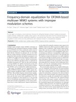
Figure 2.3: Channel Shortening Equalizer on OFDM
received sequence,

Yi = Qyi

(2.5)

= QQH ΛQQH Xi + Z
= ΛXi + Z

This is valid as long as the CIR is time invariant within the symbol duration. As
shown, only a 1-tap equalizer is needed to recover the transmitted data symbol
from the received sequence.
The long CIR is a common feature in shallow medium range UWA communication. To shorten the CIR, a time domain CSE can be applied before the FFT

operation to shorten the channel. Figure 2.3 shows the application of CSE on
OFDM. The 1-tap equalizer is generated based on the effective impulse response
which is the convolution of the CIR and the TIR.

10


Chapter 3
Time Domain Minimum Mean
Square Error Channel Shortening
Equalizers
3.1

Introduction

Figure 3.1: MMSE Channel Shortening Equalizer

The MMSE CSE is a class of equalizers that generates FIR filter that mini11


mizes the error between the output of the equalizer and the output of the TIR
in the mean square sense. The TIR is shorter than the original CIR, and in an
OFDM system, shorter than the CP. Figure 3.1 shows the block diagram of a
MMSE CSE. The design problem for MMSE CSE is to compute the equalizer
coefficients w and TIR b of a pre-defined length, such that the mean square of
the error sequence is minimized. A certain constraint is imposed on the tir and
based on this constraint the equalizer and TIR coefficients are calculated simultaneously. The vector y [m] represents the received symbols. The CIR h has l + 1
generally complex taps and is modeled as the combination of the effects of the
transmitter filter, channel distortion and front-end receiver filter.
The equalizer w is a FIR filter with Nf + 1 taps. Across a block of Nf + 1

output symbols, the input-output relationship can be presented as follow:




 h0 h1 . . . hl



 0 h h ...

y[m − 1]
0
1






 .

.
 = 



 .
.






 .
.




0 . . . 0 h0
y[m − Nf + 1]

x[m]



x[m − 1]




.
×


.




.


x[m − Nf + l]
y[m]




















0

...

0 


hl 0 . . . 



. 


. 


. 


h1 . . . hl
 
n[m]
 
 
 
n[m − 1]
 
 
 
 
.
+
 
 
.

 
 
 
.
 
 
n[m − Nf + l]









 (3.1)








12


which is the same as the matrix form:

y[m] = Hx[m] + n[m].

(3.2)

For a system with oversampling factor bigger than one, the elements in H are
vectors of length los , the oversampling factor. This becomes a fractionally spaced
equalizer scenario. The input sequence {x[m]} and the noise sequence {n[m]} are
assumed to be complex, have zero mean and are independent of each other. The
input autocorrelation matrix, Rxx is defined by
Rxx ≡ E[x[m]x[m]H ]

and the noise autocorreation matrix is,

Rnn ≡ E[n[m]n[m]H ]

Both Rxx and Rnn are assumed to be positive-definite correlation matrices.The
input-output cross-correlation and the output autocorrelation are defined as:

Rxy ≡ E[x[m]y[m]H ] = Rxx HH

(3.3)

Ryy ≡ E[y[m]y[m]H ] = HRxx HH + Rnn

(3.4)

The objective is to compute the coefficients of the equalizer w given Nb the length
of b such that the mean square of the error e[m] is minimized.
The TIR b is not restricted to be causal. This allows one extra parameter to
be introduced for better performance. A relative delay, ∆ between the equalizer

13


and the TIR is assumed. Given:

s ≡ Nf + l − ∆ − Nb

the error e[m] in Figure 3.1 can be expressed as
Nf −1

Nb −1
∗

wk ∗ y[m − k]

bj x[m − j − ∆] −

e[m] =
j=0

01×∆ b∗0 b∗1 . . . b∗Nb −1 01×s

=
−

(3.5)

k=0

∗

w0∗ w1∗ . . . wN
f −1

x[m]

y[m]

˜ H x[m] − wH y[m]
≡ b

(3.6)

Hence, the mean square error (MSE) is given by:

M SE ≡ E[|e[m]|2 ]
˜ H x[m] − wH y[m])(b
˜ H x[m] − wH y[m])H ]
= E[(b

(3.7)

˜ H Rxx b
˜ −b
˜ H Rxy w − wH Ryx b
˜ + wH Ryy w.
= b

(3.8)

By applying the orthogonality principle which states that the error is uncorrelated

with the observed data [33], we get:

E[e[m]y[m]] = 01×l
˜ H Rxy = wH Ryy
⇒b

(3.9)

14