Linearity is Strictly More Powerful than Contiguity for Encoding Graphs
Bạn đang xem bản rút gọn của tài liệu. Xem và tải ngay bản đầy đủ của tài liệu tại đây (389.35 KB, 21 trang )
Linearity is Strictly More Powerful than
,†
Contiguity for Encoding Graphs , ,
Christophe Crespelle1 , Tien-Nam Le2 , Kevin Perrot3 , and Thi Ha
Duong Phan4
1
Universit´e Claude Bernard Lyon 1 and CNRS, DANTE/INRIA,
LIP UMR CNRS 5668, ENS de Lyon, Universit´e de Lyon,
2
ENS de Lyon, Universit´e de Lyon,
3
Aix-Marseille Universit´e, CNRS, LIF UMR 7279, 13288, Marseille, France,
4
Institute of Mathematics, Vietnam Academy of Science and Technology,
18 Hoang Quoc Viet, Hanoi, Vietnam,
Abstract. Linearity and contiguity are two parameters devoted to graph
encoding. Linearity is a generalisation of contiguity in the sense that every encoding achieving contiguity k induces an encoding achieving linearity k, both encoding having size Θ(k.n), where n is the number of
vertices of G. In this paper, we prove that linearity is a strictly more
powerful encoding than linearity, i.e. there exists some graph family such
that the linearity is asymptotically negligible in front of the contiguity.
Doing so, we answer an open question asking for the worst case linearity of a cograph on n vertices: we provide an O(log n/ log log n) upper
bound which matches the previously known lower bound, then showing
that both bounds are tight.
1
Introduction
One of the most widely used operation in graph algorithms is the neighbourhood query: given a vertex x of a graph G, one wants to obtain the
list of neighbours of x in G. The classical data structure that allows to
do so is the adjacency lists. It stores a graph G in O(n + m) space, where
n is the number of vertices of G and m its number of edges, and answers
an adjacency query on any vertex x in O(d) time, where d is the degree
of vertex x. This time complexity is optimal, as long as one wants to
produce the list of neighbours of x.
†
This work was partially funded by the delegation program of CNRS.
Funding for this work was also provided by a grant from R´egion Rhˆ
one-Alpes.
This work was partially funded by the Vietnam Institute for Advanced Study in
Mathematics (VIASM).
This work was partially funded by Fondecyt Postdoctoral grant 3140527 and N´
ucleo
Milenio Informaci´
on y Coordinaci´
on en Redes (ACGO).
On the other hand, in the last decades, huge amounts of data organized
in the form of graphs or networks have appeared in many contexts such
as genomic, biology, physics, linguistics, computer science, transportation
and industry. In the same time, the need, for industrials and academics,
to algorithmically treat this data in order to extract relevant information
has grown in the same proportions. For these applications dealing with
very large graphs, a space complexity of O(n + m) is often very limiting.
Therefore, as pointed out by [11], finding compact representations of a
graph providing optimal time neighbourhood queries is a crucial issue in
practice. Such representations allow to store the graph entirely in memory while preserving the complexity of algorithms using neighbourhood
queries. The conjunction of these two advantages has great impact on the
running time of algorithms managing large amount of data.
One possible way to store a graph G in a very compact way and
preserve the complexity of neighbourhood queries is to find an order σ
on the vertices of G such that the neighbourhood of each vertex x of G is
an interval in σ. In this way, one can store the order σ on the vertices of
G and assign two pointers to each vertex: one toward its first neighbour
in σ and one toward its last neighbour in σ. Therefore, one can answer
adjacency queries on vertex x simply by listing the vertices appearing
in σ between its first and last pointer. It must be clear that such an
order on the vertices of G does not exist for all graphs G. Nevertheless,
this idea turns out to be quite efficient in practice and some compression
techniques are precisely based on it [1, 2]: they try to find orders of the
vertices that group the neighbourhoods together, as much as possible.
Then, a natural way to relax the constraints of the problem so that it
admits a solution for a larger class of graphs is to allow the neighbourhood
of each vertex to be split in at most k intervals in order σ. The minimum
value of k which makes possible to encode the graph in this way is a
parameter called contiguity [8]. Another possible way of generalization
is to use at most k orders σ1 , . . . , σk on the vertices of G such that the
neighbourhood of each vertex is the union of exactly one interval taken
in each of the k orders. This defines a parameter called the linearity of G
[4]. Linearity is a generalisation of contiguity in the sense that if a graph
G admits an encoding by contiguity k, using one linear order σ and at
most k intervals for each vertex, then one can obtain an encoding of G
by linearity k by taking k copies of σ and assigning to each vertex one of
its k intervals in each of the k copies of σ. Therefore, the linearity of a
graph is always less or equal to its contiguity.
Then the question naturally arises to know if there are some graphs for
which the linearity is significantly less than the contiguity. More formally,
are there some graph families for which the linearity is asymptotically negligible in front of the contiguity? Or are these two parameters equivalent
up to a multiplicative constant? This is the question we address here. Besides its theoretical interest, the question is also critical from a practical
point of view, as it turns out that the size of encoding by linearity and
contiguity are equivalent up to a multiplicative constant. Indeed, storing
an encoding by contiguity k requires to store a linear ordering of the n
vertices of G, i.e. a list of n integers, and the bounds of each of the k
intervals for each vertex, i.e. 2kn integers, the total size of the encoding
being (2k + 1)n integers. On the other hand, the linearity encoding also
requires to store 2kn integers for the bounds of the k intervals of each
vertex, but it needs k linear orderings of the vertices instead of just one,
that is kn integers. Thus, the total size of an encoding by linearity k is
3kn integers, instead of (2k + 1)n for contiguity k. It follows that the
two encodings have equivalent size up to a multiplicative constant. As
a consequence, since we will show that linearity can be asymptotically
negligible in front of contiguity for some graph families, and since the size
of the 2 encodings are equivalent, then linearity is strictly more powerful
than contiguity for encoding graphs.
Related work. Only little is known about contiguity and linearity of
graphs. In the context of 0 − 1 matrices, [8, 12] studied closed contiguity
and showed that deciding whether an arbitrary graph has closed contiguity at most k is NP-complete for any fixed k ≥ 2. For arbitrary graphs
again, [7] (Corollary 3.4) gave
√ an upper bound on the value of closed
contiguity which is n/4 + O( n log n). Regarding graphs with bounded
contiguity or linearity, only the class of graphs having contiguity 1, or
equivalently linearity 1, has been characterized, as being the class of
proper (or unit) interval graphs [10]. For interval graphs and permutation graphs, [4] showed that both contiguity and linearity can be up to
Ω(log n/ log log n). For cographs, a subclass of permutation graphs, [6]
showed that the contiguity can even been up to Ω(log n) and is always
O(log n), implying that both bounds are tight. The O(log n) upper bound
consequently applies for the linearity (of cographs) as well, but [6] only
provides an Ω(log n/ log log n) lower bound.
Our results. Our main result is to exhibit a family of graphs Gn on
n vertices for which the linearity of Gn is asymptotically negligible in
front of the contiguity of Gn , when n tends to infinity. In order to do
so, we prove that the linearity of a cograph G on n vertices is always
O(log n/ log log n). It turns out that this bound is tight, as it matches the
previously known lower bound on the worst-case linearity of a cograph
on n vertices [6].
2
Preliminaries.
All graphs considered here are finite, undirected, simple and loopless. In
the following, G is a graph, V (or V (G)) is its vertex set and E (or
E(G)) is its edge set. We use the notation G = (V, E) and n stands
for the cardinality |V | of V (G).An edge between vertices x and y will be
arbitrarily denoted by xy or yx. The (open) neighbourhood of x is denoted
by N (x) (or NG (x)) and its closed neighbourhood by N [x] = N (x) ∪ {x}.
The subgraph of G induced by the set of vertices X ⊆ V is denoted by
G[X] = (X, {xy ∈ E | x, y ∈ X}).
For a rooted tree T and a node u ∈ T , the depth of u in T is the number
of edges in the path from the root of T to u (the root has depth 0). The
height of T , denoted by h(T ), is the greatest depth of its leaves. We employ
the usual terminology for children, father, ancestors and descendants of a
node u in T (the two later notions including u itself), and denote by C(u)
the set of children of u. The subtree of T rooted at u, denoted by Tu , is
the tree induced by node u and all its descendants in T . A monotonic path
C of a rooted tree T is a path such that there exists some node u ∈ C
such that all nodes of C are ancestors of u. The unique node of C which
has no parent in C is called the root of the monotonic path.
In the following, the notion of minors of rooted trees is central. This
is a special case of minors of graphs (see e.g. [9]), for which we give
a simplified definition in the context of rooted trees. The contraction of
edge uv in a rooted tree T , where u is the parent of v, consists in removing
v from T and assigning its children (if any) to node u.
Definition 1. A rooted tree T is a minor of a rooted tree T if it can be
obtained from T by a sequence of edge contractions.
There are actually two notions of linearity depending on whether one
uses the open neighbourhood N (x) or closed neighbourhood N [x].
Definition 2. A closed p-line-model (resp. open p-line-model) of a graph
G = (V, E) is a tuple (σ1 , . . . , σp ) of linear orders on V such that ∀v ∈
V, ∃(I1 , . . . , Ip ) such that ∀i ∈ 1, p , Ii is an interval of σi and N [x] =
1≤i≤p Ii (resp. N (x) =
1≤i≤p Ii ).
The closed linearity (resp. open linearity) of G, denoted by cl(G) (resp.
ol(G)), is the minimum integer p such that there exists a closed p-linemodel (resp. open p-line-model) of G.
Remark 1. In the definition of a p-line-model, the set of vertices of the
intervals Ii assigned to a vertex x are not necessarily disjoint. They are
only required to cover the neighbourhood of x while being included in it.
In all the paper, we abusively extend the notion of linearity to cotrees,
referring to the linearity of their associated cograph. Moreover, we consider only closed linearity but, from the inequalities below, the bounds
we obtain (which hold up to multiplicative constants) also hold for the
open linearity. Then, for the sake of clarity, as we will not use the open
notion, in the following, we denote lin(G) instead of cl(G).
Lemma 1. For an arbitrary graph G, we have the following inequalities:
cl(G) − 1 ≤ ol(G) ≤ 2cl(G).
There are several characterizations of the class of cographs. They are
often defined as the graphs that do not admit the P4 (path on 4 vertices)
as induced subgraph. Equivalently, they are the graphs obtained from a
single vertex under the closure of the parallel composition and the series
composition. The parallel composition of two graphs G1 = (V1 , E1 ) and
G2 = (V2 , E2 ) is the disjoint union of G1 and G2 , i.e., the graph Gpar =
V1 ∪ V2 , E1 ∪ E2 . The series composition of two graphs G1 and G2 is the
disjoint union of G1 and G2 plus all possible edges from a vertex of G1 to
one of G2 , i.e., the graph Gser V1 ∪ V2 , E1 ∪ E2 ∪ {xy | x ∈ V1 , y ∈ V2 } .
These operations can naturally be extended to a finite number of graphs.
This gives a very nice representation of a cograph G by a tree whose
leaves are the vertices of the graph and whose internal nodes (non-leaf
nodes) are labelled P , for parallel, or S, for series, corresponding to the
operations used in the construction of G. It is always possible to find such
a labelled tree T representing G such that every internal node has at least
two children, no two parallel nodes are adjacent in T and no two series
nodes are adjacent. This tree T is unique [3] and is called the cotree of G.
Note that the subtree Tu rooted at some node u of cotree T also defines
a cograph, denoted Gu , and then V (Gu ) is the set of leaves of Tu . The
adjacencies between vertices of a cograph can easily be read on its cotree,
in the following way.
Remark 2. Two vertices x and y of a cograph G having cotree T are
adjacent iff the least common ancestor u of leaves x and y in T is a series
node. Otherwise, if u is a parallel node, x and y are not adjacent.
3
Linearity of a cograph and factorial rank of its cotree
In this section, we show that the linearity of a cograph is bounded by the
size of some maximal structure contained in its cotree, more precisely by
the height of a maximal double factorial tree (defined below), which we
call the factorial rank of a cotree. This result is interesting in itself as it
provides a structural explanation for the difficulty of encoding a cograph
by linearity. For our concern, the interesting point is that the number
of leaves of a double factorial tree of height h is Ω(h!). Combined with
this fact, the result presented in this section (Lemma 2) will allow us to
derive in next section the desired O(log n/ log log n) upper bound on the
linearity of cographs. We start by some necessary definitions.
Definition 3. The double factorial tree F h of height h is defined inductively as the tree whose root has 2h + 1 children u, whose subtrees Fu are
precisely F h−1 , F 0 being the unique tree of height 0 (i.e., made of a single
leaf node).
Definition 4. The factorial rank of a tree T denoted f actrank(T ), is
the maximum height of a double factorial tree being a minor of T , that is:
f actrank(T ) = max{h(T ) | T is a double factorial tree and a minor of T }.
We extend the notion of factorial rank to a node, referring to the
factorial rank of its subtree. The case where the children of node u all
have factorial rank strictly less than the one of u will play a key role.
Definition 5. Let u be a node of a tree T . If u has factorial rank k and
if all the children of u have factorial rank at most k − 1, we say that u is
minimally of factorial rank k.
We are now ready to state the result of this section, which claims that
the linearity of a cograph is linearly bounded by the factorial rank of its
cotree.
Lemma 2. Let T be a cotree and let u ∈ T of factorial rank k ≥ 0. Then,
lin(Gu ) ≤ 2k + 1. Moreover, if k ≥ 1 and u is minimally of factorial rank
k, then lin(Gu ) ≤ 2k.
Sketch of proof. We prove the result by induction. We consider an
integer k ≥ 1 such that: all nodes of factorial rank j ≤ k −1 have linearity
at most 2j + 1; and all nodes which are minimally of factorial rank k (i.e.,
whose children have factorial rank at most k − 1) have linearity at most
2k. Then, we show that any node u of factorial rank k (not necessarily
minimally) can be encoded using one more order (i.e. 2k + 1) and that
adding again one more order (i.e. using 2k + 2 orders), we can also encode
any node v which is minimally of factorial rank k + 1.
Node u of factorial rank k. In order to describe a 2k + 1-line-model
of Gu we need to distinguish different parts of Tu . Let Uk be the subset
C1
C3
u3
u1 u2
C2
C4
C6
C8
u4 u5
C5
u6 u7
C7
u9
C9
u8
Fig. 1. Example of partition into monotonic paths in the case where u is of factorial
1
rank k. The three dot circled nodes of U≤k−1 form the set U≤k−1
.
of nodes of Tu having factorial rank k and consider the set Ukmin =
{u1 , u2 , . . . , ul } Uk of its minimal elements for the ancestor relationship
(i.e. the lowest in the cotree). Note that |Ukmin | = l ≤ 2k, as otherwise u
would be of factorial rank k + 1 (since it would have 2k + 1 independent
descendants of rank 2k). By definition, all the children of the nodes of
Ukmin have factorial rank at most k − 1, and then the nodes of Ukmin
are minimally of rank k. By induction hypothesis, it follows that for all
i ∈ 1, l , ui admits a 2k-line-model for which we denote σj (ui ), with
1 ≤ j ≤ 2k, its 2k orders. We denote Tu the subtree of Tu induced by the
set of nodes Uk (by definition, Ukmin ⊆ Tu ). We also denote U≤k−1 the set
of nodes of Tu \ Tu whose parent is in Tu \ Ukmin . Nodes of U≤k−1 have, by
definition, rank at most k −1 and it follows from the induction hypothesis
that they admit a (2k − 1)-line-model. Then, for a node w ∈ U≤k−1 , we
again denote σj (w), with 1 ≤ j ≤ 2k−1, the 2k−1 orders of such a model.
In addition , we use a partition P of the nodes of Tu into l monotonic
paths Ci such that for all i ∈ 1, l , ui ∈ Ci (see Figure 1). Partition P
naturally induces a generalised partition (some parts may be empty) of
i
U≤k−1 whose parts are the subset of nodes U≤k−1
of U≤k−1 whose parent
belongs to Ci \ {ui }.
We can now describe the 2k + 1 orders (σj )1≤j≤2k+1 of the model
we build for Gu . Importantly, note that V (Gw ), w ∈ Ukmin ∪ U≤k−1 ,
is a partition of V (Gu ). In our construction, V (Gw ) will always be an
interval of σj for all w ∈ Ukmin ∪ U≤k−1 and all j ∈ 1, 2k + 1 . Then,
the description of σj is in two steps: we first give the order, denoted πj ,
in which the intervals of nodes w ∈ Ukmin ∪ U≤k−1 appear in σj and
then, for each w, we give the order, denoted σjw , in which the vertices of
Gw appear in this interval. The description of orders πj will be done by
choosing a local order on the children of each node of Uk \ Ukmin . Then πj
is defined as the unique order on Ukmin ∪ U≤k−1 respecting all the chosen
local orders, i.e. such that for any v, v ∈ Ukmin ∪ U≤k−1 , if v and v has
the same parent z and if v comes before v in the order chosen on children
of z, then all descendants of v comes before all descendants of v in πj .
To fully describe the 2k + 1-line-model of u, we must also assign to
each vertex x one interval of its neighbours in each of the orders of the
model, in such a way that these intervals entirely cover the neighbourhood
of x. In order to help our analysis, we distinguish between the external
neighbourhood of node x, which is N [x] \ V (Gw ), where w is the unique
node of Ukmin ∪ U≤k−1 being an ancestor of leaf x in Tu , and its internal
neighbourhood N [x] ∩ V (Gw ). Our construction mainly focusses on the
2k first orders of the model, which we use to encode the majority of
adjacencies of Gu , order σ2k+1 being used to encode the remaining ones.
For j ∈ 1, 2k , the purpose of order σj is to satisfy the external neighj
bourhoods of vertices of Gw for w ∈ {uj } ∪ U≤k−1
. It entirely succeeds
to do so for uj and encodes only half of the external neighbourhoods of
j
V (Gw ) for nodes w ∈ U≤k−1
, the other half being encoded in σ2k+1 . Then,
j
for each w ∈ {uj } ∪ U≤k−1
, the internal neighbourhoods of vertices of Gw
are encoded in the remaining 2k − 1 orders of (σj )1≤j≤2k . It is enough for
j
, since they admit a 2k − 1-line-model by recursion hypothesis,
w ∈ U≤k−1
but one order is missing for uj which is minimally of linearity k and is
then only guaranteed to admit a 2k-line model by recursion hypothesis.
Again, the missing order will be found in σ2k+1 .
External neighbourhoods and choice of πj ’s. Let us now show how
to choose the order πj used for defining σj such that, as claimed above,
j
most of the external adjacencies of vertices of Gw , for w ∈ {uj } ∪ U≤k−1
,
will be satisfied in σj . We choose πj the order induced by the following
local orders on the children of nodes u ∈ Uk \ Ukmin : if u is a series
node (resp. parallel node) and a strict ancestor of ui , then the child of u
which is an ancestor of uj is placed first (resp. last) in the order on the
children of u (the order on the other children of u does not matter), in all
other cases, the order on the children of u does not matter. This way, the
external neighbourhood of vertices of Guj is an interval at the end of σj
(the interval following Guj ) and this is the interval assigned to vertices of
j
Guj in σj . For nodes w ∈ U≤k−1
whose parent (which is a strict ancestor
of uj by definition) is a parallel node, the situation is the same. But for
j
nodes w ∈ U≤k−1
whose parent w is series, their external neighbourhood
is split into two intervals of σj : one following V (Gw ), which is the one we
assign to vertices of Gw in σj , and one preceding V (Gw ), denoted I
w that precede w in the order chosen for πj .
This is where we need order σ2k+1 and the partition of Tu into paths Ci
introduced earlier. To define order π2k+1 , for any node u ∈ Uk \Ukmin , we
use the same order on the children of u as the one used for πi , with i ∈
1, l such that u ∈ Ci . This ensures that for any node w ∈ U≤k−1 whose
parent w is a series node of Ci , the interval I
i
U≤k−1
) will also be an interval of σ2k+1 . This is precisely the interval
we assign to vertices of Gw in σ2k+1 , which is possible as their internal
neighbourhood will be entirely satisfied in the 2k first orders, as described
below.
Internal neighbourhoods and choice of σjw ’s. The orders σjw used for
the vertices of Gw , with w ∈ Ukmin ∪ U≤k−1 , in order σj , with j ∈ 1, 2k
are chosen as follows. For a node w ∈ U≤k−1 whose parent belong to
path Ci of the partition, if j < i (resp. if j > i) then we use the order
σj (w) (resp. σj−1 (w)), and the interval of σj associated to the vertices of
Gw is the same as the one associated to them in σj (w) (resp. σj−1 (w)).
Otherwise, if j = i the order chosen for vertices of Gw does not matter
as σj is used only for satisfying their external neighbourhood, see above.
Proceeding this way, the internal neighbourhoods of vertices of Gw are
entirely satisfied in orders (σj )j∈ 1,2k . For a node ui ∈ Ukmin , if j = i, the
order chosen on the vertices of Gui is σj (ui ) and the interval associated to
vertices of Gui in σj is the same as the one associated to them in σj (ui ).
Otherwise, if j = i, the order chosen for vertices of Gui does not matter
again as σj is used only for satisfying their external neighbourhood. Then,
only 2k − 1 orders among the 2k first ones are used to encode the internal
neighbourhoods of Gui , while the recursion hypothesis only guarantees
that lin(Gui ) ≤ 2k. For this reason, we chose the order on the vertices
of Gui in σ2k+1 as being σi (ui ), the one which was not used until now,
and the interval associated to vertices of Gui in σ2k+1 is the same as
the one associated to them in σi (ui ). This is possible as the external
neighbourhood of vertices of Gui has already been entirely satisfied before,
in order σi . Then, all adjacencies are satisfied and lin(Gu ) ≤ 2k + 1.
Node v minimally of factorial rank k +1. The only interesting case is
when v is a series node (the result is straightforward when v is parallel),
then we denote v1 , v2 , . . . , vl , with l ∈ N, the children of v, which have
factorial rank at most k by definition. From what precedes, each of them
vi admit a (2k + 1)-line-model denoted (σj (vi ))j∈ 1,2k+1 . A remarkable
property of this (2k + 1)-line-model, which we have constructed above,
is that for any vertex x, there exists an index j, later denoted ind(x),
such that the interval associated to x in σj (vi ) contains the last vertex
of σj (vi ). Based on this, the model (σj )1≤j≤2k+2 we build for Gv is as
follows. For j ∈ 1, 2k + 1 , order σj is the concatenation of orders σj (vi )
in the order from i = 1 to i = l. For any vertex x of Gvi , if j = ind(x),
the interval associated to x in σj is the same as the one associated to x
in σj (vi ); and if j = ind(x), as the interval associated to x in σind(x) (vi )
contains the last vertex of σind(x) (vi ), in the order σind(x) of the model of
Gv , we extend this interval on the right by including the vertices of Gvi
for all i > i. As v is a series node, all these vertices are indeed adjacent
to x, as well as all the vertices of Gvi for all i < i, which are the only
adjacencies of x that are not covered in the orders (σj )1≤j≤2k+1 . We use
order σ2k+2 to cover these adjacencies in the following way. For each node
vi , we choose an arbitrary order on the vertices of Gvi and concatenate
them in the order from i = 1 to i = l. Then, to any vertex x of Gvi , we
associate the interval made by all the vertices of Gvi for all i < i. This
completes the 2k + 2-model of v and the proof of the lemma.
✷
4
Main results
The first result we derive from Lemma 2 is a tight upper bound on the
worst-case linearity of cographs on n vertices. Until now, the best known
upper bound [6] was O(log n), and [6] also exhibits some cograph families
having a linearity up to Ω(log n/ log log n). Here, we show a new upper
bound of O(log n/ log log n) that matches the lower bound of [6], showing
that both bounds are therefore tight. This is a direct consequence of
Lemma 2 and of the fact that a double factorial tree of height h has
Ω(h!) vertices.
Theorem 1. For any cograph G on n vertices, we have lin(G) = O(log n/ log log n),
and this upper bound is tight.
Proof. Let T denote the cotree of G and k = f actrank(T ). From Lemma
2, the linearity of G is in O(k). Let us now show that k = O(log n/ log log n),
which will conclude this proof. According to the definition of factorial
rank, G has at least as many vertices as the double factorial tree of height
k, which has ki=0 (2i+1) vertices. It follows from Stirling’s approximation
of factorial that
√
k
(2(k + 1))!
2 π 2(k + 1) k+1
n≥
(2i + 1) = k+1
≥
e
e
2 (k + 1)!
i=0
and consequently
log n ≥ (k+1) log(k + 1) + log
2
e
+log
√
2 π
e
≥ (k+1) log(k+1)−1 .
As x ≥ y > 1 implies
x
log x
≥
y
log y ,
we have
(k + 1) log(k + 1) − 1
log n
≥
log log n
log(k + 1) + log log(k + 1) − 1
and it follows that k = O(log n/ log log n).
And finally, as [6] exhibits some cographs having linearity Ω(log n/ log log n),
consequently, the upper bound provided by the lemma is tight.
We now prove the main result aimed by this paper: linearity is a
strictly more powerful encoding than contiguity, which means, more formally, that there exists some graph families for which the linearity is
asymptotically negligible in front of the contiguity (hereafter denoted
cont(G) for a graph G). The family we exhibit is a subfamily of cographs,
which implies that the upper bound of Theorem 1 holds. Using a result of
[5] which provides a lower bound on the contiguity of cographs belonging
to this subfamily, we obtain the desired result.
Theorem 2. Let Gh , h ≥ 1, be the connected cograph whose cotree is a
complete binary tree of height h, and let n = 2h denote the number of
vertices of Gh . Then, we have lin(Gh )/cont(Gh ) = O(1/ log log n).
Proof. In [6], it is proven that cont(Gh ) = Ω(log n) and that for any
cograph G, cont(G) = O(log n). It follows that cont(Gh ) = Θ(log n).
Moreover, again in [6], it is shown that lin(Gh ) = Ω(log n/ log log n).
And we have just shown (Theorem 1 above) that for any cograph G,
lin(G) = O(log n/ log log n). It follows that lin(Gh ) = Θ(log n/ log log n)
and therefore lin(Gh )/cont(Gh ) = Θ(1/ log log n), which achieves the
proof.
5
Perspectives
In this paper, we showed that linearity provides a strictly more powerful
encoding for graphs than contiguity does, meaning that the ratio between
the contiguity and the linearity of a graph is not bounded by a constant.
To that purpose, we exhibited a graph family, namely a subfamily of
cographs, for which this ratio tends to infinity as fast as Ω(log log n),
with n the number of vertices in the graph. As a by-product of our proof,
but meaningful in itself, we also showed tight bounds for the worst-case
linearity of cographs on n vertices; tight bounds were previously known
for contiguity. Several questions naturally arises from these results and
others.
Open question 1 What is the worst case contiguity and the worst-case
linearity of arbitrary graphs?
It is straightforward to see that both of these values are bounded by
n/2, and for contiguity, [7] gave an upper bound asymptotically equivalent
to n/4. Is Ω(n) indeed the worst-case contiguity of a graph? Is the worstcase for linearity the same as the one for contiguity? Another appealing
question which is closely related is the following.
Open question 2 For arbitrary graphs, what is the maximum gap between contiguity and linearity?
In other words, let (Gn )n≥1 be a family of graphs on n vertices and
let f (n) be the ratio between the contiguity and the linearity of Gn . Can
f (n) tends to infinity faster than Ω(log log n)? What is the maximum
asymptotic growth possible for f (n)? Answering those questions would
be both theoretically and practically of key interest for the field of graph
encoding.
References
1. P. Boldi and S. Vigna. The webgraph framework I: compression techniques. In
WWW’04, pages 595–602. ACM, 2004.
2. P. Boldi and S. Vigna. Codes for the world wide web. Internet Mathematics,
2(4):407–429, 2005.
3. D.G. Corneil, H. Lerchs, and L.Stewart Burlingham. Complement reducible
graphs. Discrete Applied Mathematics, 3(3):163–174, 1981.
4. Christophe Crespelle and Philippe Gambette. Efficient neighbourhood encoding
for interval graphs and permutation graphs and O(n) breadth-first search. In
IWOCA’09, number 5874 in LNCS, pages 146–157, 2009.
5. Christophe Crespelle and Philippe Gambette. Linear-time constant-ratio approximation algorithm and tight bounds for the contiguity of cographs. In WALCOM’13, number 7748 in LNCS, pages 126–136, 2013.
6. Christophe Crespelle and Philippe Gambette. (nearly-)tight bounds on the contiguity and linearity of cographs. Theoretical Computer Science, 522:1–12, 2014.
7. C. Gavoille and D. Peleg. The compactness of interval routing. SIAM Journal on
Discrete Mathematics, 12(4):459–473, 1999.
8. P.W. Goldberg, M.C. Golumbic, H. Kaplan, and R. Shamir. Four strikes against
physical mapping of DNA. Journal of Computational Biology, 2(1):139–152, 1995.
9. L. Lov´
asz. Graph minor theory. Bulletin of the American Mathematical Society,
43(1):75–86, 2006.
10. F.S. Roberts. Representations of Indifference Relations. PhD thesis, Stanford
University, 1968.
11. G. Turan. On the succinct representation of graphs. Discr. Appl. Math., 8:289–294,
1984.
12. R. Wang, F.C.M. Lau, and Y. Zhao. Hamiltonicity of regular graphs and blocks of
consecutive ones in symmetric matrices. Discr. Appl. Math., 155(17):2312–2320,
2007.
A
Appendix : Complete proof of Lemma 2
Remark 3. The linearity of a graph is at least equal to the linearity of
any of its induced subgraphs.
Remark 4. The linearity of a cotree T whose root is a parallel node is
equal to the greatest linearity of its children.
Indeed, a p-line-model for T is simply constructed by appending the
orders of its children in any order (the first order of T is the concatenation
of the first orders of its children, the second order of T is the concatenation
of the second orders of its children, etc), and taking for each vertex the
exact same interval as in the child subtree, because there is no additional
neighbourhood to encode.
Proof of Lemma 2: We prove the result by induction. The case where
the considered node is minimally of factorial rank k is used as an intermediate in the induction. The reason is that in this particular case, we
can achieve a better encoding than the one provided in the general case,
which helps us to obtain the desired encoding for a node of factorial rank
k + 1 in the induction.
For the initialisation, we show that if u has factorial rank 0, then lin(Gu ) ≤
2 × 0 + 1 = 1. And we show that if u is minimally of factorial rank 1 (i.e.,
all its children have factorial rank 0), then lin(Gu ) ≤ 2 × 1 = 2.
For the induction step, we consider an integer k such that the statement
of the lemma holds for nodes of factorial rank at most k − 1 and for nodes
minimally of factorial rank k. Then we show that the statement still holds
for nodes of factorial rank k and for nodes minimally of factorial rank k+1.
Initialisation step.
If u has factorial rank 0, then u is a leaf of T or u is an internal node having exactly two leaf children. Then, it is straightforward that lin(Gu ) ≤ 1.
Still for the initialisation of our induction, we now show that if u has factorial rank 1 and if all its children have factorial rank at most 0, then
lin(Gu ) ≤ 2. Following remark 4, we consider that u is a series node
(otherwise, the initialisation follows from the case of factorial rank 0).
Let us denote u1 , u2 , . . . , ul the children of u. Since all the children of
u have factorial rank 0, as mentioned previously, they are either leaves
of T or internal nodes having exactly two leaf children. We consider the
case where all of them are internal nodes having two leaf children and we
denote ai , bi the two leaf children of ui , for 1 ≤ i ≤ l. We show that in this
case, the linearity of Gu is at most 2 by exhibiting a 2-line-model (σ1 , σ2 )
for Gu . As, in the other cases, we have an induced subgraph of the graph
Gu we consider here, it follows from Remark 3 that the linearity would
also be at most 2.
Arguments of this paragraph are illustrated on Figure 2. For σ1 and σ2 ,
we use the same order on the vertices of Gu , defined as σ1 = σ2 =
a1 , b1 , a2 , b2 , . . . , al , bl . For any i ∈ 1, l , the interval associated to ai in
σ1 is the set of vertices less or equal to ai in σ1 and the interval associated
to bi in σ1 is the set of vertices greater or equal to bi in σ1 . In σ2 , the interval associated to ai is the set of vertices strictly greater than bi in σ2 and
the interval associated to bi is the set of vertices strictly less than ai in σ2 .
u
S
u1 P u2 P . . . ui P . . . ul P
a1 b1 a2 b2
ai bi
σ1 : a1 , b1 , a2 , b2 , . . . , ai , bi , . . . , al , bl
σ2 : a1 , b1 , a2 , b2 , . . . , ai , bi ,. . . , al , bl
al bl
Fig. 2. Cotree of Gu (left) and example of the intervals for ai in σ1 and σ2 (right).
Induction step.
For the induction step, let us start form the hypothesis that there is an
integer k ≥ 1 such that:
– all nodes of factorial rank j ≤ k − 1 have linearity at most 2j + 1, and
– all nodes which are minimally of factorial rank k (i.e., whose children
have factorial rank at most k − 1) have linearity at most 2k.
Then, we show that all nodes u of factorial rank k have linearity at
most 2k + 1, and that all nodes v that are minimally of factorial rank
k + 1 have linearity at most 2k + 2.
Node u of factorial rank k
Figures 3, 4 and 5 picture the developments of this case. Let us start with
a node u of factorial rank k, and let us show that its linearity does not
exceed 2k + 1. Consider the set Uk of nodes of Tu that have factorial rank
k. If Uk is reduced to {u}, then u is minimally of factorial rank k and the
induction hypothesis allows to conclude without proving anything else.
Otherwise, denote Ukmin = {u1 , u2 , . . . , ul } Uk , where l ≥ 1, the subset
of nodes of Uk that are minimal for the ancestor relationship (i.e., lowest
in the cotree). By definition, these elements are incomparable for the
ancestor relationship. Then, one can build a minor of Tu , by a sequence
of edge contractions, where the set of children of u is exactly Ukmin . It
follows that |Ukmin | = l ≤ 2k, as otherwise u would be of factorial rank
k + 1. By definition again, all the children of the nodes of Ukmin have
factorial rank at most k − 1, i.e., the nodes of Ukmin = {u1 , u2 , . . . , ul }
are minimally of rank k. By induction hypothesis, it follows that for all
i ∈ 1, l , we have lin(ui ) ≤ 2k and then ui admits a 2k-line-model. We
denote σj (ui ), with 1 ≤ j ≤ 2k, the 2k orders of such a model for ui .
S
P
P
S
S
P
S
S
Fig. 3. Illustration of the case where u is of factorial rank k.
The top series node is u, and the whole cotree is Tu .
Plain nodes belong to Uk , and thick nodes (which are also plain) to Ukmin (note that
these can be leaves only for k = 0, otherwise they are series or parallel internal nodes).
The tree with plain nodes and edges is Tu and dotted nodes belong to U≤k−1 .
Dashed triangles are remaining parts of Tu : subcotrees rooted at nodes in Ukmin ∪
U≤k−1 .
In the following, we need to distinguish different parts of Tu , for which
we adopt the following notations (see Figure 3). We denote Tu the subtree
of Tu induced by the set of vertices Uk (by definition, Ukmin ⊆ Tu ).
We also denote U≤k−1 the set of nodes of Tu \ Tu whose parent is in
Tu \ Ukmin . Importantly, every vertex of Gu has exactly one ancestor
among Ukmin ∪ U≤k−1 . Note that all nodes of Tu have rank at most k,
and U≤k−1 ∩ Uk = ∅, consequently the nodes of U≤k−1 have factorial rank
at most k − 1. And by induction hypothesis, it follows that the nodes of
U≤k−1 have linearity at most 2k − 1 and then admit a (2k − 1)-line-model.
Therefore, for any node w ∈ U≤k−1 , we denote σj (w), with 1 ≤ j ≤ 2k−1,
a (2k − 1)-line-model of w.
In addition (see Figure 4), we use a partition P of the nodes of Tu
into l monotonic paths(see Section 2) denoted Ci , for 1 ≤ i ≤ l, such that
for all i, ui ∈ Ci . Partition P naturally induces a generalised partition
i
(some parts may be empty) of U≤k−1 whose parts are denoted U≤k−1
,
i
with 1 ≤ i ≤ l: U≤k−1
is the subset of nodes of U≤k−1 whose parent
belongs to Ci \ {ui }.
C1
C3
u3
u1 u2
C2
C4
u4 u5
C6
C5
u6 u7
C8
C7
u9
C9
u8
Fig. 4. Example of partition into monotonic paths in the case where u is of factorial
rank k, for the cotree of Figure 3. The three dot circled nodes of U≤k−1 form the set
1
U≤k−1
.
Construction plan The (2k + 1)-line-model we will build for Gu , denoted (σ1 , . . . , σ2k , σ2k+1 ), will be defined as the merge of two series of
2k + 1 orders, each of them defined at a different level. There will be a
low level sequence of orders, which will be “concatenated” (the formal
term is summed, see Definition 6 below) according a high level sequence
of orders.
1. First we will give, for all w ∈ Ukmin ∪ U≤k−1 , a low level sequence of
orders (σjw )j∈ 1,2k+1 on the vertices of Gw .
2. Second we will give a high level sequence of orders (πj )j∈ 1,2k+1 ,
providing for each j the relative order in which the low level orders
(σjw )w∈Ukmin ∪U≤k−1 are “concatenated” (summed).
Definition 6. The sum of orders (Ai , ≤i ) i∈X according to order (X, ≤x
) is the order ≤+ on ∪i∈X Ai , defined by a ≤+ b if and only if one of the
following holds: a, b ∈ Ai for some i and a ≤i b; or a ∈ Ai , b ∈ Aj , and
i ≤x j.
Each order σj , for j ∈ 1, 2k + 1 , will therefore be the sum of the
low level orders (σjw )w∈Ukmin ∪U≤k−1 according to the high level order πj .
To be clear, each σjw is an order on V (Gw ), and each πj is an order on
Ukmin ∪ U≤k−1 . As each vertex of Gu belongs to exactly one Gw for some
w ∈ Ukmin ∪ U≤k−1 , the sum will be an order on V (Gu ), the vertices we
are interested in.
Furthermore, we can specify the order πj locally, by providing an
order on the children of every node in Uk \ Ukmin . Naturally, The order
πj is then recursively defined using summations (the order at some node
w is the sum of its children’s orders (constructed recursively) according
to the relative order on themselves). This gives an intended order on
Ukmin ∪ U≤k−1 , because they are (by definition) exactly the children of
Uk \ Ukmin .
Note that, thanks to summations, we will have the following very
useful property: for all node w ∈ Uk ∪ U≤k−1 , and for all j ∈ 1, 2k +
1 , the vertices of Gw are an interval of σj (i.e., the vertices of Gw are
all placed next to each other). This will in particular hold for vertices
of Ukmin ∪ U≤k−1 , allowing us to exploit the induction hypothesis. To
highlight this fact, in the developments below we will refer to the vertices
of Gw in order σj for some node w in Ukmin ∪ U≤k−1 as the interval of
vertices of Gw .
We now build a (2k + 1)-line-model (σ1 , . . . , σ2k , σ2k+1 ) of Gu by
defining in the above mentioned way the orders σj . To fully describe
the model, we also need to assign to each vertex x of Gu and for each
j ∈ 1, 2k + 1 an interval of σj . In order to check that the intervals
assigned to x entirely cover its neighbourhood, we distinguish between
its internal neighbourhood and its external neighbourhood. For a node
w ∈ Ukmin ∪ U≤k−1 and a vertex x of Gw , the internal neighbourhood of x
is defined as N [x]∩V (Gw ) and its external neighbourhood as N [x]\V (Gw )
(or equivalently N (x) \ V (Gw ), as x ∈ V (Gw )).
We start the description of the model of Gu with the orders σ1 , . . . , σ2k ,
which encode the essential part of both the internal and external neighbourhoods of vertices of Gu , and we describe σ2k+1 only at the end, as it
encodes the remaining part of the adjacencies that has not been encoded
in the 2k first orders.
External neighbourhoods. Let j ∈ 1, 2k , in this paragraph, we define the order πj in which the intervals of vertices of Gw appear in σj ,
for w ∈ Ukmin ∪ U≤k−1 . If j > l, the order πj we choose does not matter,
any arbitrary order is suitable. However, if j ≤ l, the purpose of order πj
is to satisfy the external adjacencies of the vertices of Gw for any node
j
w ∈ {uj } ∪ U≤k−1
(see Figure 4). In this case, as explained above, we
define πj by choosing an order for the children of w for each node w of
Uk \Ukmin . If w is an ancestor of uj and if w is a parallel node, we choose
any order for the children of w such that the (unique) child of w which
is an ancestor of uj is the last child in the order. If w is an ancestor of
uj and w is a series node, we choose any order such that the child of w
which is an ancestor of uj is the first child of the order. And finally, if w
is not an ancestor of uj , then any order of its children is suitable for πj .
This way, all the external neighbourhood of uj (with series least common
ancestor) is on one side of σj (the pivot being the interval of vertices of
Guj ), and all the non-neighbours (with parallel least common ancestor)
are on the other side (example on Figure 5).
S
P
P
S
S
P
S
S
u6
Fig. 5. Example of order π6 , aimed at gathering in an interval the external neighbourhood of node u6 from the cotree of Figures 3 and 4. The plain circled nodes will be
placed on one side of u6 (u6 will be the first child for its ancestor series nodes), and
the dash circled nodes will be on the other side of u6 (u6 will be the last child for its
ancestor parallel nodes).
Let us now define the intervals of σj associated to vertices of Gu .
In order σj partially defined by πj above, the external neighbourhood
N (x) \ V (Guj ) of any vertex x of Guj is an interval (the same for all
vertices x of Guj ). Let us denote this latter by Iuj , it containing the last
element of σj . This Iuj is precisely the interval of σj associated to any
vertex x of Guj .
j
For a node w ∈ U≤k−1
, the situation is slightly more complicated and
we consider two cases.
– If the father of w is a parallel node, let us explain why the external
neighbourhood of vertices of Gw is an interval of σj . We denote w
the father of w, which is a parallel node and an ancestor of uj . The
external neighbourhood of w is exactly the set of leaves contained in
the other children of its series ancestors (which are all above w ). But,
as w is also an ancestor of uj , they have all been gathered into an
interval by the recursive procedure used to construct σj relatively to
uj , in an interval containing the last element of σj . We associate this
interval, denoted Iw , in σj to all vertices of Gw .
– If the father of w is a series node, then the external neighbourhood
of vertices of Gw is almost an interval of σj : including the interval of
vertices of Gw , it is an interval. Indeed, let w be the father of w, the
vertices of Gw form an interval of σj (this one includes the interval
of vertices of Gw ), and the other neighbours are placed on the same
side (the side of the last element) because the ancestors of w are also
ancestors of uj . As a result, the external neighbourhood of w is cut
into two intervals: one it precedes (denoted I
associated to all vertices of Gw in σj is Iw . The rest of the external
neighbourhood for those vertices will be covered on the additional
order σ2k+1 , defined at the end of the construction of the (2k + 1)line-model of Gu . Note that I
Internal neighbourhoods. We now concentrate on the internal neighbourhoods of vertices of Gw for nodes w ∈ Ukmin ∪ U≤k−1 , i.e., the part
of their neighbourhoods which is in Gw . To that purpose, we must precise the orders (σjw )j∈ 1,2k used on the vertices of Gw and the intervals
associated to each vertex of Gw .
– For any node ui ∈ Ukmin , with i ∈ 1, l , and all j ∈ 1, 2k ,
• if j = i, then we can take any arbitrary order for the vertices of
Guj . Indeed, the interval associated to the vertices of Guj in σj
is Iuj , as defined above in the external neighbourhood paragraph,
and it does not contain any vertex of Guj .
• If j = i, the order on the vertices of Gui is σj (ui ) and the interval
associated to vertices of Gui in σj is the same as the one associated
to them in σj (ui ).
– For a node w ∈ U≤k−1 and all j ∈ 1, 2k , the order we choose for the
vertices of Gw depends on the path Ci , with 1 ≤ i ≤ l, of the partition
P to which belongs the father of w.
• If j = i then we use any arbitrary order for the vertices of Gw .
The interval associated to the vertices of Gw in σj is Iw , as defined
above in the external neighbourhood paragraph, and again it does
not contain any vertex of Gw .
• If j < i (resp. if i < j) then we use the order σj (w) (resp. σj−1 (w)),
and the interval of σj associated to the vertices of Gw is the same
as the one associated to them in σj (w) (resp. σj−1 (w)).
i
In this way, for any i ∈ 1, l and for any w ∈ U≤k−1
, using the fact
that Gw needs only 2k−1 orders to be encoded, all the internal adjacencies
of vertices of Gw have been covered by the intervals associated to them
in orders σj , for 1 ≤ j ≤ 2k and j = i. But remember that only half of
their external adjacencies may have been covered so far (in order σi ). For
nodes ui , 1 ≤ i ≤ l, the situation is reversed: all their external adjacencies
have been covered (in order σi ), but they still need one more interval to
fully cover their internal adjacencies (because order σi (ui ) has not been
used so far). These are the reasons why we need to use one more order
σ2k+1 : in order to satisfy all these non-covered adjacencies.
Order σ2k+1 . Let us start by describing the order π2k+1 in which the
intervals of vertices of Gw appear in σ2k+1 , for w ∈ Ukmin ∪ U≤k−1 . As
before, in order to do so, we choose an order on the children of u for
each node u of Uk \ Ukmin . For each such node u there exists a unique
i ∈ 1, l such that u belongs to path Ci of partition P. The order we
choose for the children of u in π2k+1 is the same as the order used for
them in πi .
In this way, for any child w of u that belongs to U≤k−1 (and then,
i
by definition, to U≤k−1
), the interval I
Gw that have not been covered so far, is an interval of σ2k+1 (all the
missing adjacencies for w were among vertices descending from Ci ). And
this is precisely the interval associated to vertices of Gw in σ2k+1 . Note
that the order on vertices of Gw , for w ∈ U≤k−1 , does not matter in σ2k+1 ,
any arbitrary order is fine.
Now, the external adjacencies of vertices of Gw , for w ∈ U≤k−1 , are
all satisfied, but we still have to satisfy the internal adjacencies of nodes
ui , for 1 ≤ i ≤ l. To that purpose, we simply order the vertices of Gui
according to order σi (ui ), which was the only order of the 2k-line-model
of ui that we did not use so far. Each vertex of Gui is then associated in
σ2k+1 the same interval as in σi (ui ).
In this way, all the adjacencies of all the vertices of Gu are covered in
some order σj , with 1 ≤ j ≤ 2k/1. It follows that (σ1 , . . . , σ2k , σ2k+1 ) is a
(2k + 1)-line-model of Gu and therefore lin(Gu ) ≤ 2k + 1.
Node v minimally of factorial rank k + 1
In order to finish the induction step and then the proof of Lemma 2, we
now show that for a node v minimally of factorial rank k + 1 (i.e., whose
children have factorial rank at most k), we have lin(Gv ) ≤ 2k + 2.
It is straightforward to see that the linearity of the disjoint union of
two graphs is the maximum of their linearity (Remark 4). Therefore, if
v is a parallel node, its linearity is the maximum of the linearity of its
children. As in this case the children of v all have factorial rank at most
k, from what precedes, their linearity is at most 2k + 1. It follows that
lin(Gv ) ≤ 2k + 1, and then in particular lin(Gv ) ≤ 2k + 2.
Let us now consider the case where v is a series node and let us denote
v1 , v2 , . . . , vl , with l ∈ N, the children of v. From what precedes, all of them
have linearity at most 2k + 1 and for each i ∈ 1, l we have a (2k + 1)line-model of Gvi denoted (σj (vi ))j∈ 1,2k+1 . A remarkable property of
this (2k + 1)-line-model, which we have constructed above, is that for any
vertex x of Gvi , there exists an index j ∈ 1, 2k such that the interval
associated to x in σj (vi ) contains the last vertex of σj (vi ) (note that this
also holds in the initialisation step, and will still be true for the (2k + 2)line-model we are constructing now for Gv ). For each vertex x, we denote
ind(x) such an index j. We now use this property in order to construct a
(2k + 2)-line-model of Gv , which we denote (σ1 , . . . , σ2k+1 , σ2k+2 ).
For any j ∈ 1, 2k + 1 , the order σj used for v is simply the sum
(denoted +) of the orders of the (2k + 1)-line-models of its children (according to the classical order on natural integers). More explicitly, for all
j ∈ 1, 2k + 1 , we define σj as σj = σj (v1 ) + σj (v2 ) + . . . + σj (vl ). For any
i ∈ 1, l and for any vertex x of Gvi , if j = ind(x), the interval associated
to x in σj is the same as the one associated to x in σj (vi ). On the other
hand, if j = ind(x), as the interval associated to x in σind(x) (vi ) contains
the last vertex of σind(x) (vi ), in the order σind(x) of the model of Gv , we
extend this interval on the right by including the vertices of Gvi for all
i > i. As v is a series node, all these vertices are indeed adjacent to x.
In this way, for any i ∈ 1, l and for any vertex x of Gvi , the internal
neighbourhood of x is entirely covered in the orders σ1 , . . . , σ2k+1 . Regarding the external neighbourhood of x ∈ V (Gvi ), note that it can be
expressed as i ∈ 1,l and i =i V (Gvi ). The part i >i V (Gvi ) is already
covered in order σind(x) . Then, only the part i of order σ2k+2 which we define as follows. For i ∈ 1, l , we take any
arbitrary order σarb (i) on the vertices of Gvi and we build σ2k+2 as
σ2k+1 = σarb (1) + σarb (2) + . . . + σarb (l). Then, for any i ∈ 1, l and
for any vertex x of Gvi , we associate to x the interval of σ2k+2 made
of the vertices of i Thus, (σ1 , . . . , σ2k+1 , σ2k+2 ) is a (2k + 2)-line-model of Gv which is then
of linearity at most 2k + 2.
This completes the induction step and the proof of Lemma 2.
✷