Effects of Migration of Three Competing Species on Their Distributions in Multizone Environment
Bạn đang xem bản rút gọn của tài liệu. Xem và tải ngay bản đầy đủ của tài liệu tại đây (227.85 KB, 6 trang )
Effects of Migration of Three Competing
Species on Their Distributions in
Multizone Environment
Phan Thi Ha Duong
Institute of Mathematics,
Vietnam Academy of Science
and Technology,
Hanoi, Vietnam.
Email:
Doanh Nguyen-Ngoc
Abstract—In this paper, we investigate the relationship between migration and species distribution
in multizone environment. We present a discrete
model for migration of three competing species over
three zones. We prove that the migration tactics of
species leads to the fact that the system exponentially
converges to one of two typical configurations: the
first one is a case where each zone contains only one
species, the second one is a case where one species is
of density 1 in one zone, another species stays and
dominates in the two other zones, and the last species
is evenly split into the 3 zones with a density one third
in each. We also show a characterization of the initial
conditions under which the system converges to one
of the two configurations.
I.
K´evin Perrot
LIP (UMR 5668
School of Applied Mathematics,
CNRS-ENS de Lyon-UCBL1),
and Informatics,
46 alle dItalie 69364
Hanoi University of Science
Lyon Cedex 07 - France.
and Technology,
Email:
Hanoi, Vietnam.
Email:
I NTRODUCTION
An important issue in ecology is to understand
the effects of the tactics that individuals may adopt
at the population and community levels. Individuals migrate because the food is limited, they compete with others, environmental conditions are not
good for them (weather, natural calamity,...) and so
on. This leads to various portraits of distribution of
species in environment.
There was also a lot of interest in the relationship between migration of species individuals
among multizone environment and species distribution. One of the most common and simple theoretical explanation for effects of individuals’ migration
on the species distribution is ideal free distribution
(IFD) theory. The theory states that the number
of individuals that will aggregate (or else clump)
in various zones is proportional to the amount of
resources available in each. For example, if zone
1 contains twice as many resources as zone 2,
there will be twice as many individuals foraging
in zone 1 as in zone 2. The IFD theory predicts
that the distribution of individuals among zones
will minimize resource competition and maximize
fitness ( [4], [5], [6], [10], [7]).
Some recent investigations studied another factor leading to individuals’ migration and also
showed the link between the migration and the
species distribution over multizone environment
(see for examples in [2], [8], [2], [9]. The authors
showed that interaction between species leads to
migration of individuals and therefore to species
distribution. These investigations, however, take
into account only two species and two zones. The
main reason is that a model with more than two
species and two zones is much more complex and
less tractable. The aim of this work is to follow this
approach by taking into account three competing
species for territory among three zones. The raised
question is “what is the stable distribution of
the three species among three zones?” There is
no simple answer to this question. We show in
this paper that it depends on migration tactics of
individuals as well as the initial distribution of
species.
The paper is organized as follows. Section
II is dedicated to the presentation of the model.
Section III shows simulations of the model: typical
examples and remarks. Thereafter, in section IV,
we present the main results. Finally, section V is
about discussion and conclusion.
II.
zone 1
zone 2
nB1
nA2
nB2
nA3
nC1
Definition 2. The evolution rule is that if a species
dominates a zone at time t then those individuals
stay into this zone in the next time step (t + ∆t),
and if a species does not dominate a zone then in
the next time step half of them move into each of
the two other zones.
For a configuration c(t) at time t, we denote
by c(t + k∆t) the configuration obtained from c(t)
after k time steps.
P RESENTATION OF THE MODEL
nA1
the densities of the two other species in this zone.
Definition 3. A stable configuration is a configuration such that its density matrix does not change
over the time.
nC2
III.
nB3
A lot of simulations were done. We present
here three of them showing the typical stable
configurations that appear. Top of Fig. 2 shows the
nC3
zone 3
Fig. 1. Three species S = {A, B, C} and three zones Z =
{1, 2, 3}. nXi is the density of species X in zone i, X ∈
S, i ∈ Z. In the figure: density of species A in black, density
of species B in grey while density of species C in white over
three zones.
Initial configuration
A
B (0.2)
(0.5)
The system evolves in discrete time and continuous space. We consider the case of 3 species
S = {A, B, C} and 3 zones Z = {1, 2, 3} (see
Fig. 1). We call configuration at time t a distribution of the individuals of each species into the 3
zones, composed of a density nXi (t) of individuals
of species X in zone i at time t, for example
nA1 (t) is the density of individuals of species A
is zone 1 at time t, such that for every species
X : i∈Z nXi (t) = 1. Formally, a configuration
is determined by its density matrix:
nA1
nB1
nC1
nA2
nB2
nC2
nA3
nB3
nC3
(t)
(1)
If there is no ambiguity, we will usually omit the
dependence on the time t and simply refer to a notation n instead of n(t). The set of configurations
is denoted by C.
To describe the dynamics of the system, we are
going to introduce some definitions as follows:
Definition 1. In a configuration, a species dominates a zone if its density is strictly greater than
⇒ Stable configuration
(0.8)
C
n(t) =
S IMULATION
zone 1
A(0.1)
B
(0.6)
C (0.1)
zone 2
A(0.1)
B (0.45)
C
A
B
C
(1)
(1)
(1)
zone 1
zone 2
zone 3
(0.4)
zone 3
A(0.2)
A
(0.5)
A
(0.3)
B
(0.8)
B
A
(0.6)
(1)
A
B (0.1)
C
(0.4)
B (0.2)
C
(0.3)
(0.3)
(1/3)
(1/3)
(1/3)
zone 1
zone 2
zone 3
zone 1
zone 2
zone 3
A(0.1)
B
(1)
C
C
C
(0.4)
C
C
A
(0.3)
A
(0.6)
B
(0.5)
A
B
(0.55)
(0.4)
B
(0.45)
B (0.1)
C
C
(0.3)
(0.4)
C
(0.3)
(1/3)
(1/3)
(1/3)
zone 1
zone 2
zone 3
zone 1
zone 2
zone 3
C
C
Fig. 2. Three typical stable configurations. Left panel is about
initial configurations. Right panel is about the corresponding
stable configurations.
case where densities of each species are equal to 1
in one zone and are equal to 0 in the others zones.
In the middle of Fig. 2, species A is in two zones
and dominates both, species B is only in one zone
where it dominates, while species C is evenly split
into the three zones. At bottom of Fig. 2, species
A is only in one zone where it dominates, species
B is in the two others zones and dominates both,
while species C is in evenly split into the three
zones. We have the following remarks from the
above simulations:
Remark 1. There are three remarks as follows:
(1) there are two typical stable configurations: in
the first stable configuration each zone contains
only one species (top of Fig. 2), in the second
one species is of density 1 in one zone, another
species stays and dominates in the two other zones,
and the last species is evenly split into the 3
zones with a density 1/3 in each (bottom of Fig.
2); (2) the system converges rapidly to the stable
configurations; (3) it is not easy to figure out under
which conditions the system converges to one of the
two above typical configurations.
The next section is a formal analysis of these
remarks.
IV.
M AIN RESULTS
We begin in subsection IV-A by explaining that
we can discard the cases of equality in our study,
without changing the results we obtain about the
dynamic of the system, by proving that cases of
equality almost never happen. Then we describe the
two typical dynamics of the system in subsection
IV-B. Finally, subsection IV-C is devoted to the
study of the dynamics of the system according to
the initial configuration.
Firstly, we introduce some definitions as follows:
Definition 4. Let c and c be two configurations
with density matrices n and n , respectively. The
distance between the two configurations is defined
by
d(c, c ) = max {|nXi − nXi |} .
X∈S
i∈Z
Definition 5. Starting from a configuration c(t0 ),
we say that the system converges to a stable
configuration s if
∀ > 0, ∃ k( ), ∀ k > k( ) : d(c(t0 +k∆t), s) < .
Moreover, if k( ) in O log2 1 we say that the
systems exponentially converges to s.
Definition 6. We call a one-each configuration,
denoted by cOE , a configuration such that each
zone contains only one species.
Definition 7. We call a one-two configuration,
denoted by cOT , a configuration such that one
species is of density 1 in one zone, another species
stays and dominates in the two other zones, and the
last species is evenly split into the 3 zones with a
density 1/3 in each.
A. Ignoring cases of equality
We denote C ∗ the set of configurations such that
there is a case of equality between the densities of
two species competing for dominancy in a zone.
Formally,
C ∗ = {c ∈ C | ∃ X, Y, i : nXi = nY i }
where n is the density matrix of c.
Intuitively, if we consider the set C which
is uncountable (continuous space) then a case of
equality in C ∗ somehow corresponds to the restriction of an uncountably large degree of liberty to a
countable one, hence the following result holds.
Theorem 1.
|C ∗ |
|C|
= 0.
We will apply this result without explicit reference: when comparing densities of two competing
species it allows to convert an inequality into a
strict inequality.
B. Two typical behaviors
Now, we are going to show the two lemmas
about cOE and cOT .
Lemma 1 (One each). From a configuration c =
c(t0 ) such that each species X dominates exactly
one zone i, the system exponentially converges
to the stable configuration where the density of
species X in zone i is 1.
Proof: Without loss of generality, let us consider a configuration such that A dominates zone
1, B dominates zone 2 and C dominates zone 3.
First of all, we can notice that the repartition of
dominancy will never change since nXi (t + ∆t) ≥
1
2 if and only if species X dominates zone i at time
t (recall Theorem 1).
We now prove that the system exponentially
converges to the stable configuration s of density
matrix m such that
mXi =
1
0
so A dominates zone 1.
for Xi ∈ {A1, B2, C3}
otherwise
•
We can notice that
d(c(t0 +k∆t), s) = 1−
min
Xi∈{A1,B2,C3}
nXi (t0 + k∆t)
since the difference is at least as important for
species A (resp. B, C) in zone 1 (resp. 2, 3) than
in other zones. According to the repartition of
dominancy, we have
d(c(t0 + k∆t), s)
2
because half of the individuals in a zone where
they are not dominant move to their dominant zone.
Consequently, for all > 0, we have
d(c(t0 + (k + 1)∆t), s) =
d(c(t0 + k∆t), s) <
⇐⇒ k > log2
d(c, s)
which concludes the proof.
Lemma 2 (One-two). If, during two consecutive configurations c = c(t0 ) and c(t0 + ∆t), a
species X dominates zone i and another species
Y dominates the two other zones, then the system
exponentially converges to the stable configuration
s of density matrix m, defined as follows:
mXi = 1, and mXj = 0,j = i
mY i = 0, and mY j = nY j + n2Y i ,j = i
m = 1 for Z ∈
/ {X, Y }, ∀j.
Zj
3
where n is the density matrix of c.
Proof: Without loss of generality, we consider
that A dominates zone 1 and B dominates zone 2
and zone 3 and that nB2 > nB3 (let us denote this
property by (*)). We first prove that the property
(*) keeps satisfied during the evolution. For that,
it is sufficient to prove that at time t0 + 2∆t, (*)
is still satisfied, which means that if (*) is true for
two consecutive steps then it is true for the third
step, so it is true for all steps.
•
Consider zone 1, after two steps we have:
nA1 (t0 + 2∆t) = nA1 (t0 + ∆t)
0 +∆t)
≥ 12
+ 1−nA1 (t
2
nB1 (t0 + 2∆t) = 0
o +∆t)
nC1 (t0 + 2∆t) = 1−nC1 (t
≤ 12 .
2
Consider zone 2, after two steps we have:
nA2 (t0 + 2∆t) = nA3 (t0 +∆t) ≤ 1
n (t + 2∆t) = n (t2 + ∆t) 2
B2 0
B2 0
nB1 (t0 +∆t)
≥ 21
+
2
0 +∆t)
nC2 (t0 + 2∆t) = 1−nC2 (t
≤ 12 .
2
so B dominates zone 2.
•
Consider zone 3, after one step, the density
of the three species are the following:
nA2 (t0 )
nA3 (t0 + ∆t) =
2
nB3 (t0 + ∆t) = nB3 (t0 ) + nB12(t0 )
n (t + ∆t) = 1−nC3 (t0 ) .
C3 0
2
By hypothesis, we know that B dominates zone 3 after one step, then
nB3 (t0 ) + nB12(t0 ) is greater that nA22(t0 )
(t0 )
and 1−nC3
.
2
Let us consider now the situation after two
steps:
nA3 (t0 + 2∆t) = nA2 (t20 +∆t)
= nA3 (t0 ) < nB3 (t0 )
n (t + 2∆t) = n 4 (t + ∆t)
B3 0
B3 0
=
n
(t0 ) + nB12(t0 )
B3
1−n
C3 (t0 +∆t)
nC3 (t0 + 2∆t) =
2
(t0 )
= 1+nC3
.
4
We will now prove that B still dominates
zone 3 at this step, that means nB3 (t0 +
2∆t) > nC3 (t0 + 2∆t). In fact, from the
hypothesis that B dominates zone 3 at time
t0 and t0 + ∆t, we have:
nB3 (t0 ) > nC3 (t0 )
nB3 (t0 ) + nB12(t0 ) >
1−nC3 (t0 )
,
2
this implies that 4nB3 (t0 ) + nB1 (t0 )
1 + nC3 (t0 ), then nB3 (t0 + 2∆t)
nB3 (t0 ) + nB12(t0 ) > nB3 (t0 ) + nB14(t0 )
1+nC3 (t0 )
= nC3 (t0 + 2∆t).
4
We can conclude that after two steps,
dominates zone 3.
>
=
>
B
We now prove that the system exponentially
converges to the stable configuration s.
For the species B, after one step, their individ-
nA1
nB1
nC1
zone 1
uals do not move any more. For the species A, we
can apply the same argument as in Lemma 1 to
prove the exponential convergence.
We will now prove that the density of species
C in each zone exponentially converges to 13 . Let
us denote by di (t) the different nCi (t) − 13 for
i ∈ {1, 2, 3}. The density of C in zone 1 after one
step is:
nC2 (t0 ) + nC3 (t0 )
2
1 d2 (t0 ) + d3 (t0 )
= +
3
2
1 d1 (t0 )
.
= −
3
2
nC1 (t0 + ∆t) =
= −1
2 di (t0 ),
(−1)k
di (t0 ).
2k
It means that di (t0 + ∆t)
and more
This fact
generally di (t0 + k∆t) =
implies the exponential convergence for species C.
nA2
nB2
nC2
zone 2
nA3
nB3
nC3
zone 3
The first disjunction goes according to the
dominant species in zone 2:
max{nX2 (t0 )} =
X∈S
(case 1)
nA2
(case 2)
nB2
(case 3)
nC2
(case 1) We know all the dominancies, therefore we
can perform one time step. We picture c(t0 + ∆t)
below.
nA1 +
nA3
2
nB2
2
nC2 +nC3
2
zone 1
nA2 +
nA3
2
nB1
2
nC1 +nC3
2
zone 2
0
nB1 +nB2
2
nC1 +nC2
2
nB3 +
zone 3
The proof of this Lemma is then completed.
C. Dynamics of the system
The following theorem is about the portrait of
the dynamics. The theorem proves the first and
second remark of the previous section.
Theorem 2. Beginning from any configuration, the
system always converges exponentially to a cOE or
a cOT .
Proof: Let c = c(t0 ) be any configuration.
We show that after k steps with k ≥ 2, the configuration c(t0 + k∆t) will satisfies the condition
of Lemma 1 or Lemma 2, then applying those
Lemmas, one can deduce the statement of this
theorem.
To do that, we will check every possible case,
in many cases the proofs are similar. We perform a
case disjunction according to the dominant species
in each zone. The density of one species in a zone
has to be greater than any other one. Furthermore,
no species can dominate all of the three zones.
Without loss of generality, we consider that
nA1 = max{nXi }
X∈S
i∈Z
and
nB3 = max{nX3 }.
X∈S
The initial picture, where dominant densities are
boxed, is pictured below.
Species A dominates zone 1 because nA1 is the
maximal density, and nA1 is greater than nA2
which dominated over nB2 at time t0 . The comparison with C uses similar arguments. Analogously,
species B dominates zone 3.
At this stage, we perform again a case disjunction, according to the dominant species in zone 2:
(case 1.1) If A dominates zone 2, i.e.
max{nX2 (t0 + ∆t)} = nA2 + nA3 /2. Then we
X∈S
apply Lemma 2 and deduce that the system converges exponentially to a cOT .
(case 1.2) If B dominate zone 2, i.e.
max{nX2 (t0 +∆t)} = nB1 /2. This case is imposX∈S
sible. At time t0 , nC2 < nA2 and at time t0 + ∆t,
nC1 +nC3
< nB1
2
2 , then 1 = nC1 + nC2 + nC3 <
nB1 + nA2 which implies that nB1 > nA1 , a
contradiction with the maximality of nA1 .
(case 1.3) If C dominates zone 3, i.e.
max{nX2 (t0 + ∆t)} = (nC1 + nC3 )/2We apply
X∈S
Lemma 1 and deduce that the system exponentially
converges to a cOE .
(case 2) Analogously, in this case, the system
always converges exponentially to either a cOE or
a cOT .
(case 3) We apply Lemma 1 and deduce
that the system exponentially converges to a cOE .
The following theorem shows characterization
of the cases when the system converges to a cOE
(resp. cOT ).
Theorem 3. Let c be a configuration. Without loss
of generality, one can suppose that
nA1 = max{nXi } and nB3 = max{nX3 }.
X∈S
X∈S
i∈Z
Then the system exponentially converges to a cOT
if c satisfies one of the following conditions, otherwise the system exponentially converges to a cOE .
1)
nB2 = max{nX2 }
2)
nC1 +nC3
and nB2 + nB1
2 >
2
nB1
C2
and nB3 + 2 > nC1 +n
2
nA2 = max{nX2 }
and nA2 +
V.
nA3
2
>
ACKNOWLEDGMENT
This work was done while the authors were
at Vietnam Institute of Advanced Study in Mathematics (VIASM). This work was also partially
supported by the project VAST.DLT.01/12-13.
R EFERENCES
[1]
X∈S
X∈S
(density dependent) migration tactics and distribution of species over the three zones. In this study,
we just consider three species and three zones. It
would also be very interesting to take into account
of four (or in general n) species and four (or in
general n) zones (n > 4). This would lead to
a more complicated model and less tractable that
would be interesting to investigate in future work.
[2]
nC1 +nC3
2
D ISCUSSION AND C ONCLUSION
We have presented a discrete model for migration of individuals of three competing species
for territory over three zones. As a first results,
from a mathematical point of view, we have distinguished two typical stable configurations: cOE and
cOT . From an ecological point of view, we could
take into account two possibilities concerning the
species distribution: clumped distribution and uniform distribution depending on initial conditions.
Top of Fig. 2 shows a typical stable configuration where species individuals form a clumped distribution. Below, species A and B form a clumped
distribution while species C forms an uniform distribution. However, there are differences between
the two cases. In the middle of Fig. 2, species A
forms a clumped distribution over two zones while
species B forms a clumped distribution only in
the other. At bottom of Fig. 2, species A forms
a clumped distribution only in one zone while
species B forms a clumped distribution over the
two other zones.
[3]
[4]
[5]
[6]
[7]
[8]
[9]
[10]
The main conclusion that emerges from this
study is the existence of a relationship between
E. Abdllaoui, P. Auger, B. W. Kooi, R. Bravo de la Parra
and R. Mchich. Effects of density-dependent migrations on
stability of a two-patch predator-prey model. Mathematical
Biosciences, 210(1):335-354, 2007.
P. Auger, R. Bravo de la Parra, C. Poggiale, E.
Sanchez and T. Nguyen-Huu. Aggregation of variables
and applications to population dynamics. P. Magal, S.
Ruan (Eds.), Structured Population Models in Biology and
Epidemiology, Lecture Notes in Mathematics, Vol. 1936,
Mathematical Biosciences Subseries. Springer, Berlin,,
pages 209–263 , 2008.
K. Dao-Duc, P. Auger and T. Nguyen-Huu. Predator
density dependent prey dispersal in a patchy environment
with a refuge for the prey. South African Journal of
Science, pages 180–184 , 2008.
H. Dreisig. Ideal free distributions of nectar foraging
bumblebees. Oikos, 72(2), 161-172, 1995.
S. Fretwell. Populations in a Seasonal Environment.
Princeton, NJ: Princeton University Press, 1972.
R. Graeme, and S. Humphries. Multiple ideal free distributions of unequal competitors. Evolutionary Ecology
Research. 1(5): 635-640, 1999.
J. G. Godin and M. H. A. Keenleyside.Foraging on
patchily distributed prey by a chichlid fish (Teleostei
Cichlidae): a test of the ideal free distribution theory.
Animal Beaviour 32: 120-131, 1984.
D. Nguyen-Ngoc, R. Bravo de la Parra, M. A. Zavala
and P. Auger. Competition and species coexistence in
a metapopulation model: Can fast asymmetric migration
reverse the outcome of competition in a homogeneous environment. Journal of Theoretical Biology, 266, 2010,256263.
D. Nguyen-Ngoc, T. Nguyen-Huu and P. Auger. Effects
of fast density dependent dispersal on pre-emptive competition dynamics. Ecological Complexity, 26-33,10, 2012.
W. J. Sutherland, C. R. Townsend and J. M. Patmore. A
test of the ideal free distribution with unequal competitors.
Behavioral Ecology and Sociobiology. 23 (1), 51-53, 1988.