- Trang chủ >>
- Khoa Học Tự Nhiên >>
- Vật lý
DARK MATTER IN THE ECONOMICAL 3 3 1 MODEL
Bạn đang xem bản rút gọn của tài liệu. Xem và tải ngay bản đầy đủ của tài liệu tại đây (203.42 KB, 6 trang )
Proc. Natl. Conf. Theor. Phys. 36 (2011), pp. 40-45
DARK MATTER IN THE ECONOMICAL 3-3-1 MODEL
N. T. THUY, C. S. KIM
Department of Physics and IPAP, Yonsei University, Seoul 120-749, Korea
D. T. HUONG, H. N. LONG
Institute of Physics, VAST, P.O. Box 429, Bo Ho, Hanoi 10000, Vietnam
Abstract. In this work we show that the economical 3-3-1 model has a dark mater candidate. It
is a real scalar H10 in which main part is bilepton (with lepton number 2) and its mass is in the
range of some TeVs. We calculate the relic abundance of H 10 dark matter by using MicrOMEGAs
2.4 and figure out parameter space satisfying WMAP constraints.
I. INTRODUCTION
We just know only 4% particles in our universe. The dominate component (about
74%) is called dark energy and dark matter (DM) makes about 22%. The natural of DM
is still mysterious. There is no DM candidate in standard model (SM). To study DM,
we need to extend the SM. In particular, there exists a simple extension of the SM gauge
group to SU (3)C ⊗ SU (3)L ⊗ U (1)X , the so called 3-3-1 models. In this work we will
concentrate on the economical 3-3-1 model, which contains very simple Higgs sector with
two Higgs scalar triplets only. Such a scalar sector is minimal.
II. A REVIEW OF THE ECONOMICAL 3-3-1 MODEL
II.1. Particle content
The particle content in this model, which is anomaly free, is given as follows
ψaL = (νaL , laL , (νaR )c )T ∼ (3, −1/3),
T
Q1L = (u1L , d1L , UL ) ∼ (3, 1/3) ,
QαL = (dαL , −uαL , DαL )T ∼ (3∗ , 0),
uaR ∼ (1, 2/3) , daR ∼ (1, −1/3) ,
laR ∼ (1, −1),
DαR ∼ (1, −1/3) ,
UR ∼ (1, 2/3) ,
a = 1, 2, 3,
α = 2, 3,
(1)
where the values in the parentheses denote quantum numbers based on the (SU(3) L , U(1)X )
symmetry. The electric charges of the exotic quarks U and Dα are the same as of the usual
quarks, i.e., qU = 2/3, qDα = −1/3.
The spontaneous symmetry breaking in this model is obtained by two stages:
SU(3)L ⊗ U(1)X → SU(2)L ⊗ U(1)Y → U(1)Q .
The first stage is achieved by a Higgs scalar triplet with a VEV given by
1
0 T
∼ (3, −1/3) ,
χ = √ (u, 0, ω)T .
χ = χ01 , χ−
2 , χ3
2
(2)
(3)
DARK MATTER IN THE ECONOMICAL 3-3-1 MODEL
41
The last stage is achieved by another Higgs scalar triplet needed with the VEV as follows
1
0 + T
(4)
φ = φ+
∼ (3, 2/3) ,
φ = √ (0, v, 0)T .
1 , φ2 , φ3
2
The Yukawa interactions which induce masses for the fermions can be written in
the most general form:
LY = LLNC + LLNV ,
(5)
in which, each part is defined by
¯ 1L χUR + hD Q
¯ αL χ∗ DβR
LLNC = hU Q
LLNV =
αβ
l ¯
c
+hab ψaL φlbR + hνab pmn (ψ¯aL
)p (ψbL )m (φ)n
d¯
u ¯
∗
+ha Q1L φdaR + hαa QαL φ uaR + H.c.,
¯ αL χ∗ daR
¯ 1L χuaR + sdαa Q
sua Q
∗
U ¯
¯
+sD
α Q1L φDαR + sα QαL φ UR + H.c.,
(6)
(7)
where p, m and n stand for SU(3)L indices.
The VEV ω gives mass for the exotic quarks U , Dα and the new gauge bosons
Z , X, Y , while the VEVs u and v give mass for the quarks ua , da , the leptons la and all
the ordinary gauge bosons Z, W [2]. To keep a consistency with the effective theory, the
VEVs in this model have to satisfy the constraint
u2
v2
ω2 .
(8)
II.2. Stable Higgs boson
In this model, the most general Higgs potential has very simple form [3]
V (χ, φ) = µ21 χ† χ + µ22 φ† φ + λ1 (χ† χ)2 + λ2 (φ† φ)2
+λ3 (χ† χ)(φ† φ) + λ4 (χ† φ)(φ† χ).
As usual, we first shift the Higgs fields as follows:
χP1 0 + √u2
φ+
1
P0 +
φ
,
φ
=
χ=
χ−
2
2
χP3 0 + √ω2
φ+
3
√v
2
(9)
.
(10)
The subscript P denotes physical fields as in the usual treatment. Moreover, we expand
the neutral Higgs fields as
S2 + iA2
S3 + iA3
S1 + iA1
√
√
√
, φP2 0 =
, χP3 0 =
.
(11)
χP1 0 =
2
2
2
We get three massive physical particles from the Higgs sector, which are H 0 , H10 ,
and H2+ . In the effective approximation w
v, u,
H 0 ∼ S2 ,
H2+ ∼ φ+
3,
H10 ∼ S3 , G4 ∼ S1 ,
+
+
G+
G+
5 ∼ φ1 ,
6 ∼ χ2 .
(12)
H 10
From the Higgs gauge interactions given in [3], the coupling constants of
Higgs and SM
λ3 MW MX
gauge bosons depend on sζ with t2ζ = λ M 2 −λ M 2 . In the w
v, u limit, MX
MW or
1
X
2
W
42
N. T. THUY, C. S. KIM, D. T. HUONG, H. N. LONG
|t2ζ | → 0. Therefore, the H10 Higgs does not interact with the SM gauge bosons W ± , Z 0 , γ.
However, there are couplings of H10 Higgs with the Bilepton Y and Z . In order to forbid
2 ≤ M 2 . It means that 2λ ω 2 ≤ 1 g 2 ω 2 or λ ≤ 0.051.
the decay of H1o , we assume that MH
1
0
1
Y
4
1
The interactions of H10 Higgs with new gauge boson Z is Z −H10 −G3 interaction. But G3
is a Goldstone bosons, this interaction can be gauged away by a unitary transformation.
Let us consider the interaction of the dark matter to Higgs bosons. From the Higgs
potential (9), there exists the coupling of the new Higgs H10 with H 0 , H 0 . So H10 can
decay into H 0 , H 0 . The lifetime is the inversion of decay rate τ = Γ . In order to get the
constraint on the lifetime of H10 larger than our universe’s age, it is easy to see that the
value of λ3 is approximately order of 10−24 . It is to be emphasized that the limit of λ3
makes sure that tζ is small.
To avoid H10 decaying into H2+ , H2− , we need the constraint for the mass of two
2 < 4M 2 . It means that λ < λ . From the Lagrangian given in (5),
Higgs, namely MH
0
1
4
H+
1
2
it is easy to see that the H10 does not interact with the SM leptons but it interacts with
exotic quarks. As we know the exotic quarks are heavy ones, we assume that their masses
are heavier than that of H10 . In brief, to get the stable Higgs particle H10 , we need the
constraints as follows
λ1 < λ 4 ,
λ1 ≤ 0.051,
|λ3 | ∼ 10−24 ,
MH10 ≤ MU .
(13)
III. IMPLICATION FOR PARAMETER SPACE FROM WMAP
In this section, we discuss constraints on the parameter space of the 3-3-1 model
originating from the WMAP results on dark matter relic density [4]. In order to calculate
the relic density, we use micrOMEGAs 2.4 [5] after implementing new model files into
CalcHEP [6]. The parameters of our model are the self-Higgs couplings, λ 1 , λ2 , λ3 , λ4 , the
VEV w and exotic quarks masses. The relic density does not depend on λ2 and changes
a little when varying λ4 . First, we fix the values of λ2;3;4 satisfying the constraints given
in (13), especially taking λ2 = 0.12, λ3 = −10−24 , λ4 = 0.06 and varying the remaining
parameters. We consider the relic density as a function of λ1 . Fig. (1) compares the
WMAP data to the theoretical prediction. The dashed red line presents prediction by our
theory by fixing MD2 = MD3 = 100 TeV , w=10 TeV, and MU = 24 TeV. In order to meet
fully the WMAP dada, the value of λ1 must be different from the allowed value in (13).
However, if we change the mass of exotic quark, we can obtain allowed region, namely the
dot-dashed green line given by taking w = 10 TeV, MU = 36 TeV. The allowed region of
λ1 satisfy both the WMAP data and the stable Higgs constraints (13) is 0.0393 < λ 1 <
0.0406. The full orange line is obtained by fixing w = 30 TeV and MU = 36 TeV. In this
case, the constraints on λ1 is 0.0424 < λ1 < 0.0436. On the other hand, if we vary the
masses of exotic D− quarks, we can find the other allowed region of λ1 . For example, if
we take MD2 = MD3 = 12 TeV the allowed region of λ1 is 0.0502 < λ1 < 0.051. Hence,
we could conclude that the mass exotic U − quark can be larger or smaller than that of
D− quarks in order to come to agreement with the WMAP data.
Let us consider allowed region of ω, fig. (2) shows the dependence of the relic density
on the VEV w for λ1 = 0.04, λ2 = 0.12, λ3 = −10−24 , λ4 = 0.06. This figure shows that
DARK MATTER IN THE ECONOMICAL 3-3-1 MODEL
43
the VEV w < 15.33 TeV is in the WMAP-allowed region for MU = 36 TeV, MD2 = MD3
=100 TeV. However, if the values of MU = 24 TeV or MD = MU = 36 TeV, there is no
allowed region of ω in agreement with the WMAP data. It is totally difference for M U =
70 TeV and MD2 = MD3 = 12 TeV (large dashing brown line). The relic density firstly
increases then decreases as a function of w. In the WMAP band, w is in the range 8.752
- 13.85 GeV or 23.3 - 24.61 GeV.
Λ1 0.051
0.14
0.13
h2 0.1176
h2
0.12
0.11
h2 0.1064
0.10
0.09
0.08
0.00
0.02
0.04
0.06
0.08
0.10
Λ1
Fig. 1. Ωh2 vs λ1 for λ2 = 0.12, λ3 = −10−24 , λ4 = 0.06, MD2 =MD3 =100 TeV,
for w=10 TeV, MU = 24 TeV (dashed red line), for w = 10 TeV, MU = 36 TeV
(dot-dashed green line), for w = 30 TeV, MU = 36 TeV (full orange line), for MD2
= MD3 = 12 TeV, w = 10 TeV, MU = 70 TeV (large dashing brown line). Dotted
blue constant line is corresponding to λ1 = 0.051.
0.14
h2 0.1176
0.12
0.10
h2
h2 0.1064
0.08
0.06
0.04
5
10
15
20
25
30
Ω TeV
Fig. 2. Ωh2 vs w for λ1 = 0.04, λ2 = 0.12, λ3 = −10−24 , λ4 = 0.06 , for MU =
24 TeV, MD2 = MD3 = 100 TeV (dashed red line), for MU = 36 TeV, MD2 =
MD3 = 100 TeV (dot-dashed green line), for MU = MD2 = MD3 = 36 TeV (full
orange line), for MU = 70 TeV, MD2 = MD3 = 12 TeV (large dashing brown line).
The relic density increases fast when MU increases for MD2 = MD3 = 100 TeV
while it becomes flat at high values of MU for MD2 = MD3 = 12 TeV as shown in fig. (3).
The region of MU in the allowed WMAP band is 34.93 < MU < 36.73 TeV for w = 10
TeV, MD2 = MD3 = 100 TeV, 39.25 < MU < 40.89 TeV for w = 30 TeV, MD2 = MD3 =
44
N. T. THUY, C. S. KIM, D. T. HUONG, H. N. LONG
100 TeV, 66.71 < MU < 85.01 TeV for w = 10 TeV, MD2 = MD3 = 12 TeV, and 97.64
< MU < 217.8 TeV for w = 30 TeV, MD2 = MD3 = 12 TeV.
0.14
0.13
h2 0.1176
h2
0.12
0.11
h2 0.1064
0.10
0.09
50
100
150
200
250
300
MU TeV
Fig. 3. Ωh2 vs MU for λ1 = 0.04, λ2 = 0.12, λ3 = −10−24 , λ4 = 0.06, for w = 10
TeV, MD2 = MD3 = 100 TeV (dashed red line), for w = 30 TeV, MD2 = MD3 =
100 TeV (dot-dashed green line), for w = 10 TeV, MD2 = MD3 = 12 TeV (dotted
blue line), for w = 30 TeV, MD2 = MD3 = 12 TeV (full yellow line).
Next we study the variations of Ωh2 as a function of MD2 (see fig. (4)) and MD3 (see
fig. (5)). Fig. (4) shows the relic density increases to the maximum point then decreases
as MD2 increases; and the region of MD2 in the WMAP limit is 37.99 < MD2 < 259.7
TeV for MU = 36 TeV, MD3 = 100 TeV. If MU = 70 TeV, MD2 is around 12 TeV or 100
TeV for MD3 = 12 TeV, while for a larger value MD3 = 100 TeV, MD2 is around 12 TeV
or 800 TeV. ( Fig. 5) shows the variation of Ωh2 as a function MD3 . Ωh2 increases then
keeps up constant value. In case of MD2 = 12 TeV, for MU = 36 TeV, the relic density is
always below the WMAP limit, while for MU = 70 TeV, the relic density is always in the
WMAP-allowed region.
0.14
0.4
0.13
MU 36 TeV
0.12
MU 70 TeV
0.3
0.1176
h2
h2
h
2
0.11
0.2
h2 0.1064
0.10
h2 0.1176
0.1
h2 0.1064
0.09
0
200
400
600
M D2 TeV
800
1000
200
400
600
800
M D2 TeV
Fig. 4. Ωh2 vs MD2 for λ1 = 0.04, λ2 = 0.12, λ3 = −10−24 , λ4 = 0.06, w = 10
TeV, for MD3 = 100 TeV (dot-dashed green line), for MD3 = 12 TeV (dashed red
line).
1000
DARK MATTER IN THE ECONOMICAL 3-3-1 MODEL
0.14
0.12
45
0.45
h
2
0.40
MU 36 TeV
0.1176
0.35
MU 70 TeV
0.10
h2 0.1064
h2
h2
0.30
0.25
0.20
0.08
0.06
200
400
600
800
0.15
h2 0.1176
0.10
h2 0.1064
1000
200
M D3 TeV
400
600
800
1000
M D3 TeV
Fig. 5. Ωh2 vs MD3 for λ1 = 0.04, λ2 = 0.12, λ3 = −10−24 , λ4 = 0.06, w = 10
TeV, for MD2 = 100 TeV (dot-dashed green line), for MD2 = 12 TeV (dashed red
line).
IV. CONCLUSION
We have shown that the economical 3-3-1 model provides a good candidate for
dark matter called scalar Higgs H10 without any discrete symmetry; and it just requires
some constraints on Higgs couplings constant. To forbid the decay of H 10 , we require that
λ1 ≤ 0.051, λ1 < λ4 , and |λ3 | ∼ 10−24 . The parameter space has been studied in detail.
Direct and indirect searches will be studied in near future.
REFERENCES
[1]
[2]
[3]
[4]
H. N. Long, V. T. Van, J. Phys. G: Nucl. Part. Phys. 25 (1999) 2319.
P. V. Dong, D. T. Huong, Tr. T. Huong, H. N . Long, Phys. Rev. D 74 (2006) 053003.
P. V. Dong, H. N . Long, D. V. Soa, Phys. Rev. D 73 (2006) 075005.
E. Komatsu, K. M. Smith, J. Dunkley, C. L. Bennett, B. Gold, G. Hinshaw, N. Jarosik, D. Larson,
M. R. Nolta, L. Page, D. N. Spergel, M. Halpern, R. S. Hill, A. Kogut, M. Limon, S. S. Meyer, N.
Odegard, G. S. Tucker, J. L. Weiland, E. Wollack, E. L. Wright, Astrophys. J. Suppl. 192 (2011) 14
[arXiv:1001.4538 [hep-ph]].
[5] G. Belanger, F. Boudjema, P. Brun, A. Pukhov, S. Rosier-Lees, P. Salati, A. Semenov, Comput. Phys.
Commun. 182 (2011) 842 [arXiv:1004.1092 [hep-ph]].
[6] A. Pukhov, arXiv:hep-ph/0412191.
Received 30-09-2011.